


SciPy (pronounced as 'sigh pie') is a package for scientific and technical computing that builds on NumPy. With SciPy, an interactive Python session becomes as robust an environment for data processing and prototyping complex systems as MATLAB, IDL, Octave, R-Lab, and SciLab. Today, I want to briefly explain how to apply some well-known optimization algorithms in the scipy.optimize package. You can always get more detailed and up-to-date help on the functions using the help() command or by pressing Shift+Tab.
Introduction
To spare myself and the readers the need to search for and read original sources, references to method descriptions will primarily link to Wikipedia. Generally, this information is sufficient to understand the methods in broad terms and their applications. To grasp the essence of the mathematical methods, we will follow links to more authoritative publications, which can be found at the end of each article or through your favorite search engine.
The scipy.optimize module includes implementations of the following procedures:
- Constrained and unconstrained minimization of scalar functions of multiple variables (minim) using various algorithms (Nelder-Mead simplex, BFGS, Newton's conjugate gradients, and )
- Global optimization (for example, , )
- Residual minimization (least_squares) and nonlinear least squares curve fitting algorithms (curve_fit)
- Minimization of scalar functions of a single variable (minim_scalar) and root finding (root_scalar)
- Multidimensional solvers for systems of equations (root) using various methods (hybrid Powell, or large-scale methods such as ).
In this article, we will only consider the first point from this list.
Unconstrained minimization of scalar functions of multiple variables
The minim function from the scipy.optimize package provides a general interface for solving constrained and unconstrained minimization problems for scalar functions of multiple variables. To demonstrate its operation, we need a suitable multivariable function that we will minimize in various ways.
For this purpose, the Rosenbrock function of N variables is well-suited, which has the following form:

Although the Rosenbrock function and its Jacobian and Hessian matrices (first and second derivatives, respectively) are already defined in the scipy.optimize package, let’s define it ourselves.
import numpy as np

def rosen(x):
    """The Rosenbrock function"""
    return np.sum(100.0*(x[1:]-x[:-1]**2.0)**2.0 + (1-x[:-1])**2.0, axis=0)
To visualize, let’s plot in 3D the values of the Rosenbrock function from two variables.
Code for plotting
from mpl_toolkits.mplot3d import Axes3D
import matplotlib.pyplot as plt
from matplotlib import cm
from matplotlib.ticker import LinearLocator, FormatStrFormatter

# Set up a 3D plot
fig = plt.figure(figsize=[15, 10])
ax = fig.gca(projection='3d')

# Set the viewing angle
ax.view_init(45, 30)

# Create data for the plot
X = np.arange(-2, 2, 0.1)
Y = np.arange(-1, 3, 0.1)
X, Y = np.meshgrid(X, Y)
Z = rosen(np.array([X,Y]))

# Draw the surface
surf = ax.plot_surface(X, Y, Z, cmap=cm.coolwarm)
plt.show()
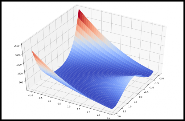
Knowing in advance that the minimum is 0 at  , let’s consider examples of how to determine the minimum value of the Rosenbrock function using various scipy.optimize procedures.
Nelder-Mead Simplex Method
Let’s assume we have an initial point x0 in 5-dimensional space. We will find the nearest point to the minimum of the Rosenbrock function using the (the algorithm is specified as the value of the method parameter):
from scipy.optimize import minimize
x0 = np.array([1.3, 0.7, 0.8, 1.9, 1.2])
res = minimize(rosen, x0, method='nelder-mead',
    options={'xtol': 1e-8, 'disp': True})
print(res.x)
Optimization terminated successfully.
Current function value: 0.000000
Iterations: 339
Function evaluations: 571
[1. 1. 1. 1. 1.]The simplex method is the simplest way to minimize a well-defined and fairly smooth function. It does not require the computation of the function's derivatives; only its values need to be specified. The Nelder-Mead method is a good choice for simple minimization tasks. However, since it does not use gradient estimates, it may take longer to find the minimum.
Powell's Method
Another optimization algorithm that only computes function values is . To use it, set method = 'powell' in the minim function.
x0 = np.array([1.3, 0.7, 0.8, 1.9, 1.2])
res = minimize(rosen, x0, method='powell',
    options={'xtol': 1e-8, 'disp': True})
print(res.x)
Optimization terminated successfully.
Current function value: 0.000000
Iterations: 19
Function evaluations: 1622
[1. 1. 1. 1. 1.]Broyden-Fletcher-Goldfarb-Shanno (BFGS) Algorithm
To achieve faster convergence to the solution, the procedure uses the gradient of the objective function. The gradient can be specified as a function or computed using first-order differences. In any case, the BFGS method typically requires fewer function calls than the simplex method.
Let's find the derivative of the Rosenbrock function in analytical form:


This expression holds for the derivatives of all variables except for the first and last, which are defined as:


Let's look at a Python function that calculates this gradient:
def rosen_der (x):
    xm = x [1: -1]
    xm_m1 = x [: - 2]
    xm_p1 = x [2:]
    der = np.zeros_like (x)
    der [1: -1] = 200 * (xm-xm_m1 ** 2) - 400 * (xm_p1 - xm ** 2) * xm - 2 * (1-xm)
    der [0] = -400 * x [0] * (x [1] -x [0] ** 2) - 2 * (1-x [0])
    der [-1] = 200 * (x [-1] -x [-2] ** 2)
    return der
The gradient computation function is specified as the value of the jac parameter in the minim function, as shown below.
res = minimize(rosen, x0, method='BFGS', jac=rosen_der, options={'disp': True})
print(res.x)
Optimization terminated successfully.
Current function value: 0.000000
Iterations: 25
Function evaluations: 30
Gradient evaluations: 30
[1.00000004 1.0000001 1.00000021 1.00000044 1.00000092]Conjugate gradient algorithm (Newton's method)
Algorithm is a modified Newton's method.
Newton's method is based on approximating the function in the local area with a second-degree polynomial:

where  is the matrix of second derivatives (Hessian matrix).
If the Hessian is positive definite, then the local minimum of this function can be found by setting the zero gradient of the quadratic form to zero. The result will be the expression:

The inverse Hessian is computed using the conjugate gradient method. An example of using this method to minimize the Rosenbrock function is given below. To use the Newton-CG method, it is necessary to specify a function that computes the Hessian.
The Hessian of the Rosenbrock function in analytical form is equal to:


where  and
and  , defines the matrix
  .
.
The other non-zero elements of the matrix are equal to:


For example, in five-dimensional space N = 5, the Hessian matrix for the Rosenbrock function has a banded form:

The code that computes this Hessian along with the code for minimizing the Rosenbrock function using the conjugate gradient method (Newton):
def rosen_hess(x):
    x = np.asarray(x)
    H = np.diag(-400*x[:-1],1) - np.diag(400*x[:-1],-1)
    diagonal = np.zeros_like(x)
    diagonal[0] = 1200*x[0]**2-400*x[1]+2
    diagonal[-1] = 200
    diagonal[1:-1] = 202 + 1200*x[1:-1]**2 - 400*x[2:]
    H = H + np.diag(diagonal)
    return H

res = minimize(rosen, x0, method='Newton-CG',
               jac=rosen_der, hess=rosen_hess,
               options={'xtol': 1e-8, 'disp': True})
print(res.x)
Optimization terminated successfully.
Current function value: 0.000000
Iterations: 24
Function evaluations: 33
Gradient evaluations: 56
Hessian evaluations: 24
[1. 1. 1. 0.99999999 0.99999999]An example of defining the Hessian matrix product and an arbitrary vector
In real-world problems, calculating and storing the entire Hessian matrix can require significant time and memory resources. In fact, it is not necessary to define the Hessian matrix itself, as only the vector equal to the product of the Hessian with another arbitrary vector is needed for the minimization procedure. Therefore, from a computational point of view, it is much preferable to immediately define a function that returns the result of the product of the Hessian with an arbitrary vector.
Let's consider the hess function, which takes the minimization vector as the first argument and the arbitrary vector as the second argument (along with other arguments of the minimized function). In our case, calculating the product of the Hessian of the Rosenbrock function with an arbitrary vector is not very difficult. If p — an arbitrary vector, then the product  takes the form:

The function that computes the product of the Hessian and an arbitrary vector is passed as the hessp argument to the minimize function:
def rosen_hess_p(x, p):
    x = np.asarray(x)
    Hp = np.zeros_like(x)
    Hp[0] = (1200*x[0]**2 - 400*x[1] + 2)*p[0] - 400*x[0]*p[1]
    Hp[1:-1] = -400*x[:-2]*p[:-2]+(202+1200*x[1:-1]**2-400*x[2:])*p[1:-1]
    -400*x[1:-1]*p[2:]
    Hp[-1] = -400*x[-2]*p[-2] + 200*p[-1]
    return Hp

res = minimize(rosen, x0, method='Newton-CG',
               jac=rosen_der, hessp=rosen_hess_p,
               options={'xtol': 1e-8, 'disp': True})
Optimization terminated successfully.
         Current function value: 0.000000
         Iterations: 24
         Function evaluations: 33
         Gradient evaluations: 56
         Hessian evaluations: 66
Trust region algorithm of conjugate gradients (Newton)
Poor conditioning of the Hessian matrix and incorrect search directions may lead to the Newton's conjugate gradient algorithm being ineffective. In such cases, preference is given to (trust-region) of Newton's conjugate gradients.
An example of defining the Hessian matrix:
res = minimize(rosen, x0, method='trust-ncg',
               jac=rosen_der, hess=rosen_hess,
               options={'gtol': 1e-8, 'disp': True})
print(res.x)
Optimization terminated successfully.
Current function value: 0.000000
Iterations: 20
Function evaluations: 21
Gradient evaluations: 20
Hessian evaluations: 19
[1. 1. 1. 1. 1.]Example with the product of the Hessian and an arbitrary vector:
res = minimize(rosen, x0, method='trust-ncg',
                jac=rosen_der, hessp=rosen_hess_p,
                options={'gtol': 1e-8, 'disp': True})
print(res.x)
Optimization terminated successfully.
Current function value: 0.000000
Iterations: 20
Function evaluations: 21
Gradient evaluations: 20
Hessian evaluations: 0
[1. 1. 1. 1. 1.]Krylov-type methods
Similar to the trust-ncg method, Krylov-type methods are well-suited for solving large-scale problems as they only use matrix-vector products. Their essence lies in solving the problem within a trust region bounded by the truncated Krylov subspace. For indefinite problems, this method is preferable since it requires fewer nonlinear iterations due to a smaller number of matrix-vector products per subproblem compared to the trust-ncg method. Additionally, the solution to the quadratic subproblem is found more accurately than with the trust-ncg method.
An example of defining the Hessian matrix:
res = minimize(rosen, x0, method='trust-krylov',
               jac=rosen_der, hess=rosen_hess,
               options={'gtol': 1e-8, 'disp': True})

Optimization terminated successfully.
         Current function value: 0.000000
         Iterations: 19
         Function evaluations: 20
         Gradient evaluations: 20
         Hessian evaluations: 18

print(res.x)

    [1. 1. 1. 1. 1.]
Example with the product of the Hessian and an arbitrary vector:
res = minimize(rosen, x0, method='trust-krylov',
               jac=rosen_der, hessp=rosen_hess_p,
               options={'gtol': 1e-8, 'disp': True})

Optimization terminated successfully.
         Current function value: 0.000000
         Iterations: 19
         Function evaluations: 20
         Gradient evaluations: 20
         Hessian evaluations: 0

print(res.x)

    [1. 1. 1. 1. 1.]
Approximate solution algorithm in the trust region
All methods (Newton-CG, trust-ncg, and trust-krylov) are well-suited for solving large-scale problems (with thousands of variables). This is due to the underlying conjugate gradient algorithm that implies an approximate computation of the inverse Hessian matrix. The solution is found iteratively, without explicit decomposition of the Hessian. Since it only requires the function for the product of the Hessian and an arbitrary vector, this algorithm is particularly effective for sparse (band diagonal) matrices. This ensures low memory costs and significant time savings.
In medium-sized problems, the costs for storing and factoring the Hessian are not critical. This means that a solution can be achieved in fewer iterations by solving the trust region subproblems almost exactly. To do this, some nonlinear equations are solved iteratively for each quadratic subproblem. Such a solution typically requires 3 or 4 Cholesky decompositions of the Hessian matrix. As a result, the method converges in fewer iterations and requires fewer function evaluations than other implemented trust region methods. This algorithm only involves the definition of the full Hessian matrix and does not support the ability to use the product function of the Hessian and an arbitrary vector.
Example with minimizing the Rosenbrock function:
res = minimize(rosen, x0, method='trust-exact',
               jac=rosen_der, hess=rosen_hess,
               options={'gtol': 1e-8, 'disp': True})
res.x
Optimization terminated successfully.
Current function value: 0.000000
Iterations: 13
Function evaluations: 14
Gradient evaluations: 13
Hessian evaluations: 14
array([1., 1., 1., 1., 1.])Let's pause here. In the next article, I will try to share the most interesting aspects of conditional minimization, the application of minimization in solving approximation problems, minimizing a single-variable function, arbitrary minimizers, and finding the roots of a system of equations using the scipy.optimize package.
Source:
Source: habr.com
