

Introduction to Operating Systems
Hello, Habr! I would like to present to your attention a series of translation articles of some interesting literature in my opinion — OSTEP. This material dives deeply into the workings of Unix-like operating systems, specifically — working with processes, various schedulers, memory, and other similar components that make up a modern OS. You can view the original materials here . Please note that the translation is done non-professionally (rather freely), but I hope I preserved the overall meaning.
Laboratory work on this subject can be found here:
Other parts:
You can also check out my channel on =)
Introduction to the Scheduler
The Essence of the Problem: How to Develop a Scheduler Policy
How should the basic frameworks of scheduler policies be designed? What key assumptions must be made? What metrics are important? What basic techniques were used in early computing systems?
Workload Assumptions
Before discussing possible policies, let's first make a few simplifying digressions about the processes running in the system, collectively known as workload. Defining workload as a critical part of policy building and the more you know about the load, the better quality policy you can write.
Let’s make the following assumptions about the processes running in the system, sometimes referred to as jobs (tasks). Almost all of these assumptions are unrealistic, but necessary for the development of thought.
- Each task runs for the same amount of time,
- All tasks are submitted at the same time,
- The submitted task runs until completion,
- All tasks use only the CPU,
- The runtime of each task is known.
Scheduler Metrics
In addition to some assumptions about the load, we also need a tool to compare different scheduling policies: scheduler metrics. A metric is simply a measure of something. There are several metrics that can be used to compare schedulers.
For example, we will use a metric called turnaround time Turnaround time for a task is defined as the difference between the completion time of the task and the time the task arrived in the system.
Tturnaround=Tcompletion−Tarrival
Since we assumed that all tasks arrived at the same time, then Ta=0 and thus Tt=Tc. This value will naturally change when we alter the assumptions mentioned above.
Another metric is fairness. Performance and fairness are often opposing characteristics in scheduling. For example, a scheduler may optimize for performance at the cost of delaying other tasks, thereby reducing fairness. FIRST IN FIRST OUT (FIFO)
The simplest algorithm we can implement is called FIFO or
The most basic algorithm we can implement is called FIFO or first come (in), first served (out). This algorithm has several advantages: it is very simple to implement and fits all our assumptions, performing the task quite well.
Let's consider a simple example. Suppose 3 tasks were set simultaneously. But let's assume task A arrived slightly earlier than the others, so it will be listed before the others, just as task B will be in relation to task C. Let's assume each of them will take 10 seconds to complete. What would be the average completion time of these tasks in this case?
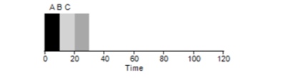
By calculating the values — 10+20+30 and dividing by 3, we get an average execution time of the program as 20 seconds.
Now let's try to change our assumptions. In particular, assumption 1, and thus we will no longer assume that each task takes the same amount of time. How will FIFO perform this time?
As it turns out, different execution times for tasks have a very negative impact on the productivity of the FIFO algorithm. Suppose task A takes 100 seconds, while tasks B and C still take 10 seconds each.
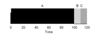
As shown in the figure, the average time for the system will be (100+110+120)/3=110. This effect is called the convoy effect, where some short-term consumers of a resource will line up behind a heavy user. It's like waiting in line at a grocery store when there’s a customer in front of you with a full cart. The best solution to the problem is to try to switch lines or just relax and take deep breaths.
Shortest Job First
Is there a way to resolve such a situation with heavyweight processes? Of course. Another type of scheduling is calledShortest Job First (SJF). Its algorithm is also quite primitive — as the name suggests, the shortest tasks will be executed first, one after another.
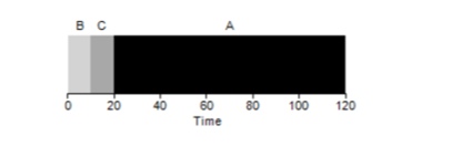
In this example, the result of running the same processes will improve the average turnaround time of the programs, and it will be 50 instead of 110, which is almost 2 times better.
Thus, under the given assumption that all tasks arrive at the same time, the SJF algorithm seems to be the most optimal one. However, our assumptions still do not appear realistic. This time, let's modify assumption 2 and assume that tasks can arrive at any time, rather than all at once. What problems could this lead to?
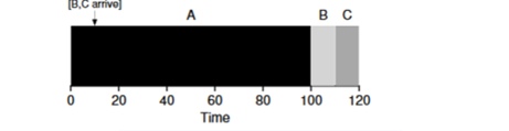
Let's say task A (100s) arrives first and starts executing. At time t=10, tasks B and C arrive, each of which will take 10 seconds. Thus, the average execution time is (100+(110-10)+(120-10))/3 = 103. What could the scheduler do to improve the situation?
Shortest Time-to-Completion First (STCF)
To improve the situation, let's drop assumption 3 that the program runs and works until completion. In addition, we will need hardware support and, as you might guess, we will use a timer to interrupt the running task and context switching. This way, the scheduler can take action at the moment tasks B and C arrive—stop executing task A, process tasks B and C, and after they finish, continue executing process A. Such a scheduler is called STCFor Preemptive Job First.
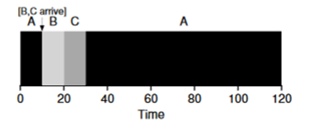
The result of this scheduler’s operation will be: ((120-0)+(20-10)+(30-10))/3=50. Thus, this scheduler becomes even more optimal for our tasks.
Response Time Metric
Thus, if we know the execution times of the tasks and that these tasks only use the CPU, STCF will be the best solution. And at one time, these algorithms worked quite well. However, now users spend most of their time at the terminal and expect productive interactive responses from it. Thus, a new metric was born— response time .
Response time is calculated as follows:
Tresponse=Tfirstrun−Tarrival
Thus, for the previous example, the response times will be: A=0, B=0, C=10 (abg=3.33).
It turns out that the STCF algorithm is not very effective in situations where three tasks arrive simultaneously — it has to wait until the smaller tasks have fully completed. Thus, the algorithm is good for turnaround time metrics, but poor for interactivity metrics. Imagine sitting at a terminal trying to type characters in an editor and having to wait more than 10 seconds because another task is occupying the CPU. That's not very pleasant.
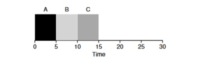
This brings us to another problem — how can we build a scheduler that is responsive to response time?
Round Robin
To solve this problem, an algorithm was developed Round Robin (RR). The main idea is quite simple: instead of running tasks to completion, we will run a task for a certain amount of time (called a time quantum) and then switch to another task in the queue. The algorithm continues to work until all tasks are completed. Additionally, the runtime should be a multiple of the time after which the timer interrupts the process. For example, if the timer interrupts the process every x = 10ms, then the execution window size must be a multiple of 10 and can be 10, 20, or x*10.
Consider an example: Tasks A, B, and C arrive simultaneously in the system, and each wants to run for 5 seconds. The SJF algorithm would execute each task to completion before starting another. In contrast, the RR algorithm with a time slot of 1s would progress through the tasks as follows (see Fig. 4.3):
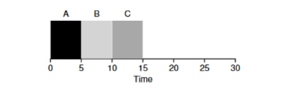
(SJF Again (Bad for Response Time)
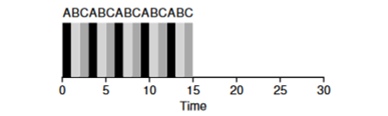
(Round Robin (Good For Response Time)
The average response time for the RR algorithm is (0+1+2)/3=1, whereas for SJF it is (0+5+10)/3=5.
It is logical to assume that the time slice is a very important parameter for RR; the shorter it is, the higher the response time. However, it should not be too small, as the context-switching time also plays a role in overall performance. Thus, the choice of execution time slice is set by the OS architect and depends on the tasks that are planned to be executed in it. Context switching is not the only overhead that consumes time — a running program also operates on various caches, and with each switch, it is necessary to save and restore this environment, which can also take a considerable amount of time.
RR is an excellent scheduler if we're only talking about response time metrics. But how will the turnaround time metric behave with this algorithm? Let's consider the example above, where tasks A, B, and C each run for 5 seconds and arrive at the same time. Task A will finish at 13 seconds, B at 14 seconds, and C at 15 seconds, resulting in an average turnaround time of 14 seconds. Therefore, RR is the worst-performing algorithm for turnaround time metrics.
In general terms, any RR-type algorithm is fair; it divides CPU time equally among all processes. Thus, these metrics constantly conflict with each other.
Consequently, we have several opposing algorithms and still several assumptions remain — that the task time is known and that the task only uses the CPU.
Mixing with I/O
First, let’s remove assumption 4, which states that the process only uses the CPU; this is naturally not the case, as processes can also interact with other hardware.
At the moment when a process requests an I/O operation, it transitions to a blocked state, waiting for the completion of the I/O. If the I/O is sent to a hard disk, such an operation may take several milliseconds or longer, and during this time, the CPU will be idle. The scheduler can then assign the CPU to any other process. The next decision the scheduler must make is when the process will finish its I/O. When this happens, an interrupt will occur, and the OS will transition the I/O-requesting process to a ready state.
Let's consider an example with several tasks. Each of them requires 50ms of CPU time. However, the first task will access I/O every 10ms (which will also be executed in 10ms). Meanwhile, process B simply uses 50ms of CPU time without any I/O.
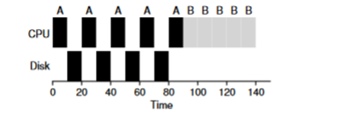
In this example, we will use the STCF scheduler. How will the scheduler behave if we run process A on it? It will proceed as follows: first, it will fully complete process A, and then process B.
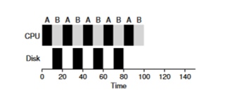
The traditional approach to solving this problem is to interpret every 10ms subtask of process A as a separate task. Thus, when starting with the STJF algorithm, the choice between the 50ms task and the 10ms task is clear. Once subtask A completes, process B and the I/O will be initiated. After I/O is finished, the 10ms process A will be restarted instead of process B. This allows for overlapping, where the CPU is used by another process while the first one waits for I/O. As a result, the system is better utilized — at the moment when interactive processes are waiting for I/O, other processes can run on the CPU.
The oracle is gone.
Now let's try to eliminate the assumption that the execution time of a task is known. This is overall the worst and most unrealistic assumption on the list. In fact, in average operating systems, the OS usually knows very little about task execution times, so how can one build a scheduler without knowing how long a task will run? Perhaps we could use some principles of RR to address this issue?
Summary
We have looked at the basic ideas of task scheduling and examined two families of schedulers. The first runs the shortest task first, thereby improving turnaround time, while the second evenly splits time among all tasks, improving response time. Both algorithms perform poorly in situations where the algorithms from the other family excel. We also considered how parallel use of CPU and I/O can enhance performance, but we still did not solve the problem of OS foresight. In the next session, we will explore a scheduler that looks into the near past and tries to predict the future, called the multi-level feedback queue.
Source: habr.com
