

Good day.
In recent years, I have dedicated myself to researching and developing various algorithms for spatial signal processing in adaptive antenna arrays, and I continue to work on this in my current job. Here, I would like to share the knowledge and tips I have discovered. I hope this will be useful for those beginning to study this field of signal processing or simply interested in it.
What is an adaptive antenna array?
is a set of antenna elements arranged in some manner in space. Simplifying, the structure of the adaptive antenna array that we will consider can be represented as follows:
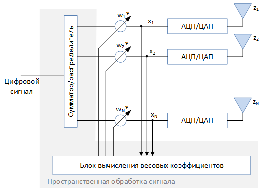
Adaptive antenna arrays are often referred to as 'smart' antennas (). What makes an antenna array 'smart' is the signal processing block and the algorithms implemented within it. These algorithms analyze the received signal and form a set of weighting coefficients $inline$w_1…w_N$inline$, which determine the amplitude and initial phase of the signal for each of the elements. The specified amplitude-phase distribution determines of the entire array as a whole. The ability to synthesize a radiation pattern of the desired shape and modify it during signal processing is one of the main features of adaptive antenna arrays, allowing them to solve a wide . But let’s go in order.
How is the radiation pattern formed?
characterizes the signal power radiated in a certain direction. For simplicity, let's assume the elements of the array are isotropic, i.e., for each of them the power of the radiated signal does not depend on direction. The increase or decrease of power radiated by the array in a certain direction results from of electromagnetic waves emitted by various elements of the antenna array. A stable interference pattern for electromagnetic waves is only possible under the condition of their , i.e., the phase difference of the signals must not change over time. Ideally, each of the elements of the antenna array should emit at the same carrier frequency $inline$f_{0}$inline$. However, in practice, we have to deal with narrowband signals that have a finite bandwidth spectrum $inline$Delta f << f_{0}$inline$.
Let all elements of the array emit the same signal with $inline$x_n(t)=u(t)$inline$. Then at the receiver, the signal received from the n-th element can be represented in form:
$$display$$a_n(t) = u(t-tau_n)e^{i2pi f_0(t-tau_n)}$$display$$
where $inline$tau_n$inline$ is the delay in signal propagation from the antenna element to the receiving point.
Such a signal is “quasiharmonic”, and to meet the coherence condition, the maximum delay in EM wave propagation between any two elements must be much less than the characteristic envelope time change of the signal $inline$T$inline$, i.e. $inline$u(t-tau_n) ≈ u(t-tau_m)$inline$. Thus, the condition for the coherence of a narrowband signal can be written as follows:
$$display$$T≈frac{1}{Delta f}>>frac{D_{max}}{c}=max(tau_k-tau_m) $$display$$
where $inline$D_{max}$inline$ is the maximum distance between the elements of the array, and $inline$c$inline$ is the speed of light.
When receiving a signal, coherent summation is performed in digital form in the spatial processing block. In this case, the complex value of the digital signal at the output of this block is determined by the expression:
$$display$$y=sum_{n=1}^Nw_n^*x_n$$display$$
The last expression is more conveniently represented as of N-dimensional complex vectors in matrix form:
$$display$$y=(textbf{w},textbf{x})=textbf{w}^Htextbf{x}$$display$$
where w and x — column vectors, and $inline$(.)^H$inline$ is the .
Vector representation of signals is one of the fundamentals when working with antenna arrays, as it often allows avoiding cumbersome mathematical derivations. Moreover, identifying the received signal at a given moment in time with a vector often allows one to abstract from the real physical system and understand what is happening from a geometric perspective.
To calculate the radiation pattern of an antenna array, one must mentally and sequentially "launch" a set of from all possible directions. In this case, the values of the elements of the vector x can be represented as follows:
$$display$$x_n=s_n=exp{-i(textbf{k}(phi,theta),textbf{r}_n)}$$display$$
where k – , $inline$phi$inline$ and $inline$theta$inline$ – and , characterizing the direction of arrival of the plane wave, $inline$textbf{r}_n$inline$ – coordinate of the antenna element, $inline$s_n$inline$ – element of the phasor vector tr1 != str2 of the plane wave with the wave vector k (in English literature, the phasor vector is referred to as the steerage vector). The dependency of the square of the amplitude on y $inline$phi$inline$ and $inline$theta$inline$ defines the antenna array's directivity pattern for reception given a weight vector w.
Characteristics of the antenna array's directivity pattern
It is convenient to study the general properties of the directivity pattern of antenna arrays on a linear equidistant antenna array in the horizontal plane (i.e., the directivity pattern depends only on the azimuthal angle $inline$phi$inline$). This is convenient from two perspectives: analytical calculations and visual representation.
Let's calculate the directivity pattern for a unit weight vector ($inline$w_n=1, n = 1 … N$inline$), following the described approach.
The mathematics here
The projection of the wave vector onto the vertical axis: $inline$k_v=-frac{2pi}{lambda}sinphi$inline$
The vertical coordinate of the antenna element with index n: $inline$r_{nv}=(n-1)d$inline$
Here d – the period of the antenna array (the distance between adjacent elements), λ — wavelength. All other elements of the vector r are equal to zero.
The signal received by the antenna array is expressed as follows:
$$display$$y=sum_{n=1}^{N}1 ⋅exp{i2pi nfrac{d}{lambda}sinphi}$$display$$
We will apply the formula for and :
$$display$$y=frac{1-exp{i2pi Nfrac{d}{lambda}sinphi}}{1-exp{i2pi frac{d}{lambda}sinphi}}=frac{sin(pi frac{Nd}{lambda}sinphi)}{sin(pi frac{d}{lambda}sinphi)}exp{ipi frac{d(N-1)}{lambda}sinphi}$$display$$
In the end, we will get:
$$display$$F(phi)=|y|^2=frac{sin^2(pi frac{Nd}{lambda}sinphi)}{sin^2(pi frac{d}{lambda}sinphi)} $$display$$
Periodicity of the directivity pattern
The obtained directivity pattern of the antenna array is a periodic function of the sine of the angle. This means that at certain values of the ratio d/λ it has diffraction (additional) maxima.
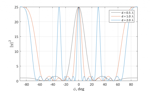 Unnormalized directivity pattern of the antenna array for N = 5
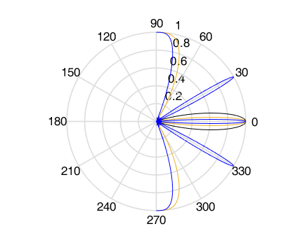 Normalized directivity pattern of the antenna array for N = 5 in polar coordinates
The position of the "diffraction maxima" can be directly observed from the for the radiation pattern. However, we will try to understand where they physically and geometrically come from (in N-dimensional space).
attribute vector tr1 != str2 are complex exponents $inline$e^{iPsi n}$inline$, the values of which are determined by the generalized angle $inline$Psi = 2pi frac{d}{lambda}sinphi$inline$. If there are two generalized angles corresponding to different directions from which a plane wave arrives, for which $inline$Psi_1 = Psi_2 + 2pi m$inline$, then this means two things:
- Physically: the flat wave fronts arriving from these directions induce identical amplitude-phase distributions of electromagnetic oscillations on the elements of the antenna array.
- Geometrically: for these two directions coincide.
Directions of wave arrival related in this way are equivalent in terms of the antenna array and indistinguishable from each other.
How to determine the angular region in which there is always only one principal maximum of the radiation pattern? We will do this in the vicinity of the zero azimuth based on the following considerations: the amount of phase advance between two neighboring elements must lie in the interval from $inline$-pi$inline$ to $inline$pi$inline$.
$$display$$-pi<2pifrac{d}{lambda}sinphi<pi$$display$$
Solving this inequality gives us a condition for the uniqueness region near zero:
$$display$$|sinphi|<frac{lambda}{2d}$$display$$
It is evident that the size of the uniqueness region in angle depends on the ratio d/λ. If d = 0.5λ, so each direction of signal arrival is 'individual', and the uniqueness region covers the full range of angles. If d = 2.0λ, then the directions 0, ±30, ±90 are equivalent. Diffraction lobes appear in the radiation pattern.
Typically, diffraction lobes are suppressed using directional antenna elements. In this case, the complete radiation pattern of the antenna array is the product of the radiation pattern of one element and the array of isotropic elements. The parameters of the radiation pattern of one element are usually chosen based on the condition for the uniqueness region of the antenna array.
The width of the main lobe
The engineering formula for estimating the width of the main lobe of an antenna system is: $inline$Delta phi ≈ frac{lambda}{D}$inline$, where D is the characteristic size of the antenna. This formula is applicable to various types of antennas, including parabolic ones. We will show that it is also valid for antenna arrays.
We will define the width of the main lobe by the first nulls of the radiation pattern near the main maximum. The numerator for $inline$F(phi)$inline$ becomes zero at $inline$sinphi=mfrac{lambda}{dN}$inline$. The first nulls correspond to m = ±1. $inline$frac{lambda}{dN}<<1$inline$, we get $inline$Delta phi = 2frac{lambda}{dN}$inline$.
Typically, the width of the antenna pattern's radiation pattern is defined by the -3 dB half-power level. In this case, the expression used is:
$$display$$Delta phi≈0.88frac{lambda}{dN}$$display$$
Example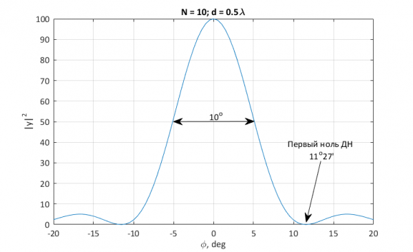
The width of the main lobe can be controlled by assigning different amplitude values to the weighting coefficients of the antenna array. Let's consider three distributions:
- Uniform amplitude distribution (weights 1): $inline$w_n=1$inline$.
- Amplitude values decreasing towards the edges of the array (weights 2): $inline$w_n=0.5+0.3cos(2pifrac{n-1}{N}-pifrac{N-1}{N})$inline$.
- Amplitude values increasing towards the edges of the array (weights 3): $inline$w_n=0.5-0.3cos(2pifrac{n-1}{N}-pifrac{N-1}{N})$inline$.
The figure shows the resulting normalized radiation patterns on a logarithmic scale: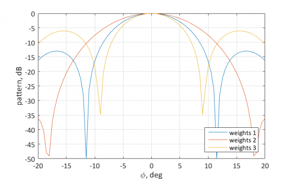
From the figure, the following trends can be observed: a decreasing amplitude distribution towards the edges of the array leads to a widening of the main lobe of the radiation pattern, but a reduction in the level of side lobes. Conversely, increasing amplitude values towards the edges of the antenna array lead to a narrowing of the main lobe and an increase in the level of side lobes. Here it is convenient to consider limiting cases:
- The amplitude of the weighting coefficients for all elements except the edge ones is zero. The weights for the edge elements are equal to one. In this case, the array becomes equivalent to a two-element antenna array with a period of D = (N-1)d. It is not difficult to estimate the width of the main lobe using the formula provided above. In this case, the side lobes will turn into diffraction maxima and will align in level with the main maximum.
- The weight of the central element is equal to one, and all others are zero. In this case, we essentially have a single antenna with an isotropic radiation pattern.
Direction of the main maximum
So, we have looked at how to adjust the width of the main lobe of the directional pattern. Now, let's see how to control the direction. Let’s recall for the accepted signal. Suppose we want the maximum of the directional diagram to be pointed in a certain direction $inline$phi_0$inline$. This means that maximum power should be received from that direction. The corresponding phase vector is $inline$textbf{s}(phi_0)$inline$ in N-dimensional vector space, and the received power is determined as the square of the scalar product of this phase vector with the weight coefficient vector. wThe scalar product of two vectors is maximized when they are , i.e., $inline$textbf{w}=beta textbf{s}(phi_0)$inline$, where β is some normalization factor. Thus, if we choose the weight vector equal to the phase vector for the desired direction, we will rotate the maximum of the directional pattern.
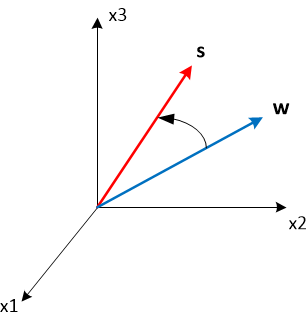
As an example, let's consider the following weight coefficients: $inline$textbf{w}=textbf{s}(10°)$inline$
$$display$$w_n=exp{i2pifrac{d}{lambda}(n-1)sin(10pi/180)}$$display$$
As a result, we will obtain a directional diagram with the main maximum in the direction of 10°.
Now let's apply the same weight coefficients, but not for signal reception, but for transmission. Here it is worth noting that when transmitting a signal, the direction of the wave vector changes to the opposite. This means that the elements for reception and transmission differ in sign in the exponent, i.e., they are related by complex conjugation. As a result, we will obtain a maximum of the directional pattern for transmission in the direction of -10°, which does not coincide with the reception maximum using the same weight coefficients. To correct the situation, it is necessary to apply the complex conjugation to the weight coefficients as well.
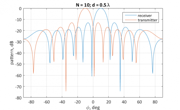
This particular feature of forming the directional pattern for reception and transmission should always be kept in mind when working with antenna arrays.
Let’s play with the directional diagram
Multiple maxima
Let’s set a task to form two main maxima of the directional pattern in the directions: -5° and 10°. To do this, we will choose a weighted sum of the phase vectors for the corresponding directions as the weight vector.
$$display$$textbf{w}=betatextbf{s}(10°)+(1-beta)textbf{s}(-5°)$$display$$
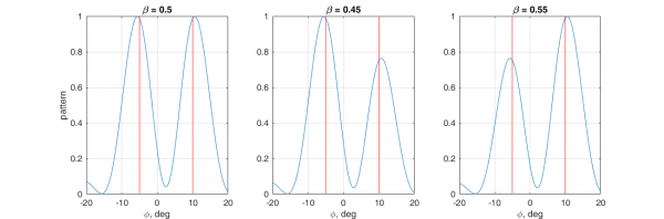 By adjusting the ratio β you can control the relationship between the main lobes. It’s convenient to observe what happens in vector space. If β greater than 0.5, the weight vector lies closer to tr1 != str2(10°), otherwise to tr1 != str2(-5°). The closer the weight vector is to one of the phasors, the greater the corresponding scalar product, and consequently the magnitude of the corresponding maximum of the directional pattern.
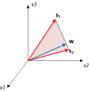
However, it should be noted that both main lobes have a finite width, and if we want to align with two close directions, these lobes will merge into one, oriented towards some average direction.
One maximum and zero
Now let’s try to set the maximum of the directional diagram to the direction $inline$phi_1=10°$inline$ and simultaneously suppress the signal coming from the direction $inline$phi_2=-5°$inline$. To do this, it is necessary to set the directional pattern to zero for the corresponding angle. This can be done as follows:
$$display$$textbf{w}=textbf{s}_1-frac{textbf{s}_2^Htextbf{s}_1}{N}textbf{s}_2$$display$$
where $inline$textbf{s}_1 = textbf{s}(10°)$inline$, and $inline$textbf{s}_2 = textbf{s}(-5°)$inline$.
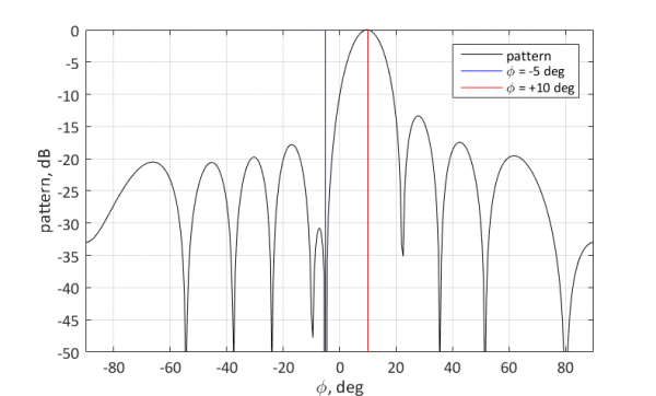
The geometric meaning of choosing the weight vector is as follows. We want this vector w to have the maximum projection on $inline$textbf{s}_1$inline$ while being orthogonal to the vector $inline$textbf{s}_2$inline$. The vector $inline$textbf{s}_1$inline$ can be represented as the sum of two components: a collinear vector to $inline$textbf{s}_2$inline$ and a vector orthogonal to $inline$textbf{s}_2$inline$. To meet the requirements of the task, it is necessary to choose the second component as the weight coefficient vector w. The collinear component can be calculated by projecting the vector $inline$textbf{s}_1$inline$ onto the normalized vector $inline$frac{textbf{s}_2}{sqrt{N}}$inline$ using the scalar product.
$$display$$textbf{s}_{1||}=frac{textbf{s}_2}{sqrt{N}}frac{textbf{s}_2^Htextbf{s}_1}{sqrt{N}}$$display$$
Consequently, by subtracting the collinear component from the original phasor vector $inline$textbf{s}_1$inline$, we obtain the desired weight vector.

Some additional remarks
- Earlier, I overlooked the question of normalizing the weight vector, i.e., its length. However, the normalization of the weight vector does not affect the characteristics of the antenna array's radiation pattern: the direction of the main lobe, the width of the main lobe, etc. It can also be shown that this normalization does not affect the output of the spatial processing block. Therefore, when considering signal spatial processing algorithms, a unit normalization of the weight vector is typically assumed, i.e. $inline$textbf{w}^Htextbf{w}=1$inline$.
- The ability to form the radiation pattern of an antenna array is determined by the number of elements N. The more elements there are, the greater the possibilities. There are more degrees of freedom in implementing spatial weight processing, allowing for more ways to 'rotate' the weight vector in N-dimensional space.
- In receiving, the radiation pattern of an antenna array physically does not exist; it only exists in the 'imagination' of the computational unit processing the signal. This means that several radiation patterns can be synthesized simultaneously, enabling independent processing of signals coming from different directions. The situation is a bit more complicated for transmission, but it is also possible to synthesize multiple radiation patterns to transmit different data streams. This technology in communication systems is known as .
- With the provided MATLAB code, you can experiment with radiation patterns on your own.
Code% antenna array settings N = 10; % number of elements d = 0.5; % period of antenna array wLength = 1; % wavelength mode = 'receiver'; % receiver or transmitter % weights of antenna array w = ones(N,1); % w = 0.5 + 0.3*cos(2*pi*((0:N-1)-0.5*(N-1))\/N).'; % w = 0.5 - 0.3*cos(2*pi*((0:N-1)-0.5*(N-1))\/N).'; % w = exp(2i*pi*d\/wLength*sin(10\/180*pi)*(0:N-1)).'; % b = 0.5; w = b*exp(2i*pi*d\/wLength*sin(+10\/180*pi)*(0:N-1)).' + (1-b)*exp(2i*pi*d\/wLength*sin(-5\/180*pi)*(0:N-1)).'; % b = 0.5; w = b*exp(2i*pi*d\/wLength*sin(+3\/180*pi)*(0:N-1)).' + (1-b)*exp(2i*pi*d\/wLength*sin(-3\/180*pi)*(0:N-1)).'; % s1 = exp(2i*pi*d\/wLength*sin(10\/180*pi)*(0:N-1)).'; % s2 = exp(2i*pi*d\/wLength*sin(-5\/180*pi)*(0:N-1)).'; % w = s1 - (1\/N)*s2*s2'*s1; % w = s1; % normalize weights w = w.\/sqrt(sum(abs(w).^2)); % set of angle values to calculate pattern angGrid_deg = (-90:0.5:90); % convert degree to radian angGrid = angGrid_deg * pi \/ 180; % calculate set of steerage vectors for angle grid switch (mode) case 'receiver' s = exp(2i*pi*d\/wLength*bsxfun(@times,(0:N-1)',sin(angGrid))); case 'transmitter' s = exp(-2i*pi*d\/wLength*bsxfun(@times,(0:N-1)',sin(angGrid))); end % calculate pattern y = (abs(w'*s)).^2; %linear scale plot(angGrid_deg,y\/max(y)); grid on; xlim([-90 90]); % log scale % plot(angGrid_deg,10*log10(y\/max(y))); % grid on; % xlim([-90 90]);
What tasks can be solved using adaptive antenna arrays?
Optimal reception of an unknown signalIf the direction of the incoming signal is unknown (and in cases where the communication channel is multi-path, there can be several directions), by analyzing the signal received by the antenna array, it is possible to form an optimal weight vector w so that the output OSH of the spatial processing block is maximized.
Optimal reception of a signal in the presence of noiseHere, the task is set as follows: the spatial parameters of the expected useful signal are known, however, there are sources of interference in the external environment. It is necessary to maximize the OSH of the AR output while minimizing the impact of interference on signal reception.
Optimal signal transmission to the userThis task is addressed in mobile communication systems (4G, 5G) as well as in Wi-Fi. The essence is simple: using special pilot signals in the user's feedback channel, the spatial characteristics of the communication channel are evaluated, and based on this, an optimal weight coefficient vector for transmission is selected.
Spatial multiplexing of data streamsAdaptive antenna arrays allow for data transmission to multiple users simultaneously on the same frequency, creating an individual radiation pattern for each of them. This technology is called MU-MIMO and is currently being actively implemented (and in some places already) in communication systems. The capability for spatial multiplexing is included, for instance, in the 4G LTE mobile communication standard, Wi-Fi standard IEEE802.11ay, and 5G mobile communication standards.
Virtual antenna arrays for radarsDigital antenna arrays allow the formation of a virtual antenna array substantially larger in size using several transmitting antenna elements for signal processing. The virtual array has all the characteristics of a real one, but requires fewer hardware resources for its implementation.
Estimation of radiation source parametersAdaptive antenna arrays enable the estimation of the number, power, sources of radio radiation, establishing a statistical relationship between signals from various sources. The main advantage of adaptive antenna arrays in this regard is the ability to super-resolve closely spaced sources of radiation. Sources where the angular distance is less than the width of the main lobe of the antenna array's radiation pattern (). This is mainly made possible by the vector representation of the signal, a well-known signal model, as well as the apparatus of linear mathematics.
Thank you for your attention
Source: habr.com
