Richard Hamming: Chapter 13. Information Theory

We did it!

The aim of this course is to prepare you for your technical future.

Hello, Habr. Remember the awesome article You and your work (+219, 2588 bookmarked, 429k reads)?

So, Hamming (yes, yes, self-checking and self-correcting Hamming codes) has a whole book, based on his lectures. We're translating it because the guy knows his stuff.

This book is not just about IT; it's about the mindset of incredibly cool people. It's not just about positive thinking; it describes the conditions that increase the chances of doing great work.

Thanks to Andrey Pakhomov for the translation.

Information Theory was developed by C. E. Shannon in the late 1940s. The Bell Labs management insisted that he call it 'Communication Theory,' as it is a much more accurate title. For obvious reasons, the name 'Information Theory' has a significantly greater impact on the public, so Shannon chose it, and it’s what we know it as today. The very name suggests that the theory deals with information, which makes it important as we delve deeper into the information age. In this chapter, I will touch on some key conclusions from this theory, providing not strict, but rather intuitively understandable proofs of some individual propositions of this theory, so you understand what 'Information Theory' really is, where you can apply it, and where you can't.

First of all, what is 'information'? Shannon identifies information with uncertainty. He chose the negative logarithm of the probability of an event as the quantitative measure of the information you gain when an event with probability p occurs. For example, if I tell you that it is foggy in Los Angeles, then p is close to 1, which basically doesn't give us much information. But if I say that it's raining in Monterey in June, then there will be uncertainty in this statement, and it will contain more information. A certain event contains no information at all, since log 1 = 0.

Let's delve into this in more detail. Shannon believed that a quantitative measure of information should be a continuous function of the probability of an event p, and for independent events, it should be additive—the amount of information received from two independent events should equal the amount of information received from their joint occurrence. For instance, the outcomes of rolling dice and flipping a coin are typically considered independent events. Let's translate the above into mathematical language. If I (p) is the amount of information contained in an event with probability p, then for a joint event consisting of two independent events x with probability p1 and y with probability p2, we have

(x and y are independent events)

This is Cauchy's functional equation, true for all p1 and p2. To solve this functional equation, let’s assume that

p1 = p2 = p,

this gives

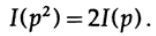
If p1 = p2 and p2 = p, then

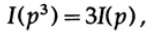
and so on. By extending this process using the standard method for exponentials, for all rational numbers m / n, the following holds true

From the assumed continuity of the information measure, it follows that the logarithmic function is the only continuous solution to Cauchy's functional equation.

In information theory, it is customary to take the logarithm base to be 2, so a binary choice contains exactly 1 bit of information. Therefore, information is measured by the formula

Let's pause and clarify what happened above. Firstly, we did not define the concept of 'information'; we merely established the formula for its quantitative measure.

Secondly, this measure depends on uncertainty, and while it adequately suits machines—for instance, telephone systems, radio, television, computers, etc.—it does not reflect the normal human relationship with information.

Thirdly, this is a relative measure; it depends on your current state of knowledge. If you are looking at a stream of 'random numbers' from a random number generator, you assume that each subsequent number is uncertain. However, if you know the formula for generating 'random numbers', the next number will be known and, consequently, will not contain information.

Thus, the definition given by Shannon for information applies in many cases to machines, but seems to not correspond to human understanding of the word. This is precisely why the 'Theory of Information' should have been called the 'Theory of Communication.' However, it is already too late to change definitions (which contributed to the initial popularity of the theory, and which still lead people to think that this theory deals with 'information'), so we must come to terms with them, but you should clearly understand how far Shannon's definition of information is from its common meaning. Shannon's information deals with something entirely different, namely uncertainty.

Here is what you need to consider when proposing any terminology. How closely does the proposed definition, for example, Shannon's definition of information, align with your initial idea and how much does it differ? Almost no term perfectly reflects your prior vision of the concept, but ultimately, the terminology used conveys the meaning of the concept, so formalizing something through clear definitions always introduces some noise.

Consider a system whose alphabet consists of symbols q with probabilities pi. In this case, the average amount of information in the system (its expected value) equals:

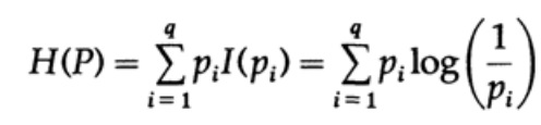
This is called the entropy of the system with the probability distribution {pi}. We use the term 'entropy' because the same mathematical form arises in thermodynamics and statistical mechanics. This is why the term 'entropy' creates an aura of importance that is ultimately not justified. The identical mathematical form of the expression does not imply the same interpretation of the symbols!

The entropy of the probability distribution plays a central role in coding theory. Gibbs' inequality for two different probability distributions pi and qi is one of the important consequences of this theory. So, we must prove that

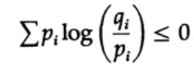
The proof relies on the obvious graph, Fig. 13.I, which shows that

and equality is achieved only when x = 1. We apply the inequality to each term of the sum from the left side:

If the communication system's alphabet consists of q symbols, then by assuming the probability of transmitting each symbol q_i = 1/q and substituting q, we derive from Gibbs's inequality.

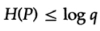
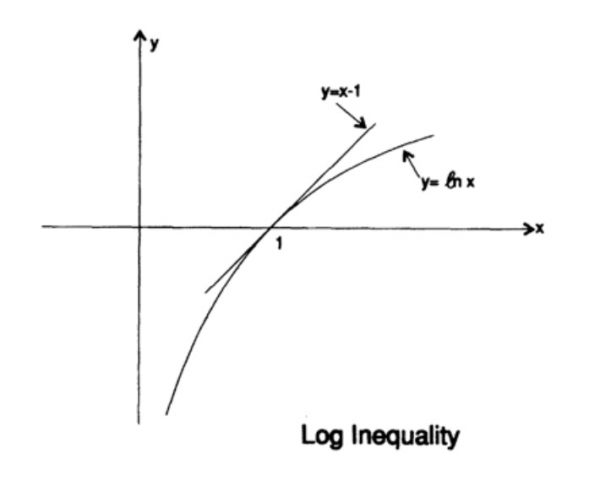
Figure 13.I

This indicates that if the probability of transmitting all q symbols is the same and equals 1/q, then the maximum entropy is ln q; otherwise, the inequality holds.

In the case of a uniquely decodable code, we have Kraft's inequality.

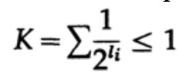
Now, if we define pseudo-probabilities

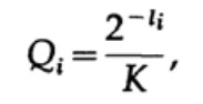
where it is finite 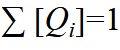= 1, which follows from Gibbs's inequality,

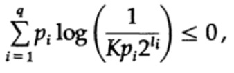
and applying a bit of algebra (remember that K ≤ 1, so we can drop the logarithmic term, possibly strengthening the inequality later), we get

where L is the average length of the code.

Thus, entropy serves as a lower bound for any symbol-by-symbol code with an average code word length L. This is Shannon's theorem for a noiseless channel.

Now consider the main theorem regarding the limitations of communication systems, where information is transmitted as a stream of independent bits and noise is present. It is implied that the probability of correctly transmitting one bit P > 1/2, and the probability that the bit's value will be inverted during transmission (an error occurs) equals Q = 1 - P. For convenience, assume that the errors are independent and the probability of error is the same for each transmitted bit—that is, there is 'white noise' in the communication channel.

We have a long stream of n bits encoded into a single message—an n-dimensional expansion of a one-bit code. The value of n will be defined later. Consider a message consisting of n bits as a point in n-dimensional space. Since we have n-dimensional space—and for simplicity, let's assume that each message has the same probability of occurrence—there are M possible messages (M will also be defined later), thus the probability of any sent message is

(sender)
Graph 13.II

Next, let's discuss the concept of channel capacity. Without going into details, channel capacity is defined as the maximum amount of information that can be reliably transmitted over a communication channel, considering the use of the most efficient coding. There is no argument that more information can be transmitted through a communication channel than its capacity. This can be proven for a binary symmetric channel (which we are using in our case). The capacity of the channel, when sending bit by bit, is given as

where, as before, P is the probability of no error in any transmitted bit. When sending n independent bits, the channel capacity is defined as

If we are close to the channel capacity, then we should send almost that amount of information for each of the symbols ai, i = 1, …, M. Considering that the probability of occurrence of each symbol ai is equal to 1 / M, we obtain

when we send any of the M equally probable messages ai, we have

When sending n bits, we expect the occurrence of nQ errors. In practice, for a message consisting of n bits, we will have approximately nQ errors in the received message. For large n, the relative variation (variation = width of the distribution, )
of the number of errors will become increasingly narrow as n increases.

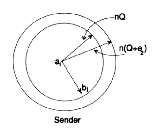
Thus, from the transmitter's side, I take message ai to send and draw a sphere around it with a radius

that is slightly larger by an amount equal to e2 than the expected number of errors Q, (see Figure 13.II). If n is sufficiently large, there is an arbitrarily small probability that the message point bj on the receiver's side lies outside this sphere. Let's illustrate the situation as I see it from the transmitter's perspective: we have any radius from the transmitted message ai to the received message bj with an error probability equal to (or nearly equal to) a normal distribution achieving its peak at nQ. For any given e2, there exists an n large enough that the probability that the received point bj lying outside my sphere will be as small as you wish.

Now let's consider the same situation from your perspective (Fig. 13.III). On the receiver's side, there is a sphere S(r) of the same radius r around the received point bj in n-dimensional space, such that if the received message bj is inside my sphere, then the message I sent ai is inside your sphere.

How can an error occur? An error can happen in the cases described in the table below:

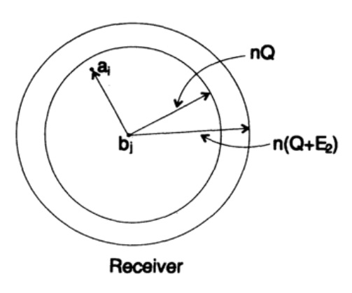
Figure 13.III

Here we see that if there exists at least one more point within the sphere constructed around the received point that corresponds to a possible sent uncoded message, then an error has occurred during transmission, as you cannot determine which of these messages was sent. The sent message contains no errors only if the point corresponding to it is within the sphere, and no other possible points in this code are located within the same sphere.

We have a mathematical equation for the probability of an error Pe if the message ai was sent.

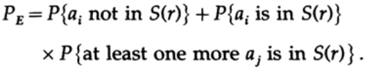
We can discard the first factor in the second term, assuming it to be 1. Thus we obtain an inequality.

It is evident that

therefore

we apply again to the last term on the right

Assuming n is large enough, the first term can be made arbitrarily small, say, less than some number d. Therefore we have

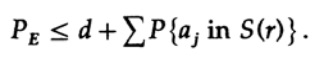
Now let’s consider how one can construct a simple substitution code for encoding M messages consisting of n bits. Without any idea of how to construct the code (error correction codes had not yet been invented), Shannon chose random coding. Flip a coin for each of the n bits in the message and repeat the process for M messages. In total, nM coin flips need to be made, so there are

codeword dictionaries, each with an equal probability of ½nM. Of course, the random process of creating a code dictionary means that there is a chance of duplicates appearing as well as code points that will be close to each other, and therefore will be sources of probable errors. It needs to be proven that if this does not happen with a probability greater than any chosen small error level, then the given n is large enough.
The crucial point is that Shannon averaged all possible codebooks to find the average error! We will use the symbol Av [.] to denote the average value over a multitude of all possible random code dictionaries. Averaging over the constant d, of course, gives a constant since, for averaging, each term coincides with any other term in the sum.

which can be increased (M–1 becomes M)

For any specific message, by averaging all codebooks, the encoding runs through all possible values, so the average probability that a point is in the sphere is the ratio of the volume of the sphere to the total volume of the space. The volume of the sphere is then

where s=Q+e2 <1/2 and ns must be an integer.

The last term on the right is the largest in this sum. First, we will estimate its value using Stirling's formula for factorials. Then we will examine the reduction coefficient of the preceding term, noting that this coefficient increases when moving left, so we can: (1) bound the value of the sum by the sum of a geometric series with this initial coefficient, (2) extend the geometric series from ns terms to an infinite number of terms, (3) calculate the sum of the infinite geometric series (standard algebra, nothing substantial), and finally obtain the limiting value (for sufficiently large n):

Note how the entropy H(s) appeared in the binomial identity. Notice that the Taylor series expansion H(s)=H(Q+e2) provides an estimate obtained by considering only the first derivative and ignoring all the rest. Now, let's assemble the final expression:

where

All we need to do is choose e2 such that e3 < e1, and then the last term can be made arbitrarily small for sufficiently large n. Therefore, the average error PE can be made arbitrarily small with a channel capacity that is as close to C as needed.
If the average value across all codes has a sufficiently small error, then at least one code must be suitable, meaning there exists at least one appropriate encoding system. This is an important result derived by Shannon — the 'Shannon theorem for noisy channels,' though it should be noted that he proved this for a much more general case than the simple binary symmetric channel I used. For the general case, the mathematical derivations are much more complex, but the ideas are not that different, so it is often possible to reveal the true meaning of the theorem through the example of a specific case.

Let’s critique the result. We have repeatedly said: 'With sufficiently large n.' But how large does n need to be? Very, very large, if you really want to be simultaneously close to the channel capacity and be confident in the correct transmission of data! So large that you will effectively be forced to wait a very long time to accumulate a message made up of that many bits, in order to subsequently encode it. At the same time, the size of the random code dictionary will be simply enormous (after all, such a dictionary cannot be represented in a shorter form than a full list of all Mn bits, given that n and M are very large)!

Error correction codes avoid waiting for a very long message, with its subsequent encoding and decoding through very large code books, because they circumvent code books altogether and instead use ordinary computations. In simple theory, such codes tend to lose the ability to approach the channel capacity while maintaining a sufficiently low error rate, but when a code corrects a large number of errors, they can yield good results. In other words, if you allocate some channel capacity for error correction, you should use that correction capability most of the time, i.e., each transmitted message should have a large number of errors corrected; otherwise, you are wasting that capacity.

Nevertheless, the theorem proven above is not meaningless! It demonstrates that efficient transmission systems must use carefully designed encoding schemes for very long bit strings. An example includes satellites that have ventured beyond the outer planets; as they move away from the Earth and the Sun, they are forced to correct an increasing number of errors in the data block: some satellites use solar panels that provide about 5 watts, while others use atomic power sources that give approximately the same power. The weak power of the source, the small size of the transmitter dishes, and the limited dimensions of the receiver dishes on Earth, along with the vast distance that the signal must traverse—all these factors require the use of high-error-correction codes to build an effective communication system.

Let us return to the n-dimensional space we used in the proof above. In discussing it, we showed that almost the entire volume of a sphere is concentrated around its outer surface—thus, it is almost certain that the transmitted signal will be located at the surface of the sphere constructed around the received signal, even with a relatively small radius of such a sphere. Therefore, it is not surprising that the received signal, after correcting for an arbitrarily large number of errors, nQ, turns out to be as close as desired to the error-free signal. The channel capacity we considered earlier is key to understanding this phenomenon. Note that such spheres constructed for Hamming codes with error correction do not overlap. A large number of nearly orthogonal dimensions in n-dimensional space explains why we can fit M spheres in space with minimal overlap. If we allow for a small, arbitrarily negligible overlap, which may only lead to a small number of errors during decoding, we can achieve a dense arrangement of spheres in space. Hamming guaranteed a certain level of error correction, Shannon—low error probability—while maintaining actual throughput as close to the channel capacity as possible, which Hamming codes cannot achieve.

Information theory does not explain how to design an efficient system, but it points the way toward effective communication systems. It is a valuable tool for building communication systems between machines, yet, as previously mentioned, it has little relevance to how people exchange information with one another. The extent to which biological inheritance is similar to technical communication systems is simply unknown, so at this point, it is unclear how applicable information theory is to genes. We have no choice but to try, and if success reveals a machine-like nature to this phenomenon, then failure will indicate other significant aspects of the nature of information.

Let’s briefly digress. We have seen that all initial definitions, to a greater or lesser extent, must express the essence of our original beliefs, but they carry a certain degree of distortion and therefore prove inapplicable. Traditionally, it is thought that ultimately, the definition we use actually defines the essence; however, this merely indicates how we should process things and does not carry any real meaning for us. The postulation approach, which is highly endorsed in mathematical circles, leaves much to be desired in practice.

Now we will examine an example of IQ tests, where the definition is as cyclic as you wish, and consequently misleads you. A test is created that is supposed to measure intelligence. It is later reviewed to make it as consistent as possible, and then it is published and calibrated in a straightforward manner so that the measured 'intelligence' turns out to be normally distributed (of course according to the calibration curve). All definitions must be rechecked, not only when they are first proposed, but also much later when they are used in conclusions drawn. To what extent are the boundaries of definitions suitable for the task at hand? How often do definitions given in one context begin to be applied in sufficiently different contexts? This happens quite frequently! In the humanities, which you will inevitably encounter in your life, this occurs more often.

Thus, one of the goals of this presentation on information theory, aside from demonstrating its usefulness, was to warn you about this danger, or to show you exactly how to use it to achieve the desired outcome. It has long been noted that initial definitions greatly influence what you ultimately find, much more than it seems. Initial definitions require your close attention not only in any new situation but also in areas you have long worked in. This will help you understand to what degree the results obtained are tautological rather than something useful.

A well-known story by Eddington tells of people who were fishing in the sea with a net. After examining the size of the fish they caught, they determined the minimum size of the fish that can be found in the sea! Their conclusion was dictated by the tool they used, not by reality.

To be continued…

Anyone who wants to help with the translation, layout, and publication of the book—please contact me privately or at magisterludi2016@yandex.ru

By the way, we have also launched the translation of another cool book — “The Dream Machine: A History of the Computer Revolution”)

We are especially looking for those who can help translate the bonus chapter that is only available on video. (we translate for 10 minutes, the first 20 have already been taken)

Table of contents and translated chaptersPreface

1. Intro to The Art of Doing Science and Engineering: Learning to Learn (March 28, 1995) Translation: Chapter 1
2. “Foundations of the Digital (Discrete) Revolution” (March 30, 1995) Chapter 2. Foundations of the Digital (Discrete) Revolution
3. “History of Computers — Hardware” (March 31, 1995) Chapter 3. History of Computers — Hardware
4. “History of Computers — Software” (April 4, 1995) Chapter 4. History of Computers — Software
5. “History of Computers — Applications” (April 6, 1995) Chapter 5. History of Computers — Practical Applications
6. “Artificial Intelligence — Part I” (April 7, 1995) Chapter 6. Artificial Intelligence — I
7. “Artificial Intelligence — Part II” (April 11, 1995) Chapter 7. Artificial Intelligence — II
8. “Artificial Intelligence III” (April 13, 1995) Chapter 8. Artificial Intelligence — III
9. “n-Dimensional Space” (April 14, 1995) Chapter 9. n-Dimensional Space
10. “Coding Theory — The Representation of Information, Part I” (April 18, 1995) Chapter 10. Coding Theory — I
11. “Coding Theory — The Representation of Information, Part II” (April 20, 1995) Chapter 11. Coding Theory — II
12. «Error-Correcting Codes» (April 21, 1995) Chapter 12. Error-Correcting Codes
13. «Information Theory» (April 25, 1995) Chapter 13. Information Theory
14. «Digital Filters, Part I» (April 27, 1995) Chapter 14. Digital Filters — 1
15. «Digital Filters, Part II» (April 28, 1995) Chapter 15. Digital Filters — 2
16. «Digital Filters, Part III» (May 2, 1995) Chapter 16. Digital Filters — 3
17. «Digital Filters, Part IV» (May 4, 1995) Chapter 17. Digital Filters — IV
18. «Simulation, Part I» (May 5, 1995) Chapter 18. Simulation — I
19. «Simulation, Part II» (May 9, 1995) Chapter 19. Simulation — II
20. «Simulation, Part III» (May 11, 1995) Chapter 20. Simulation — III
21. «Fiber Optics» (May 12, 1995) Chapter 21. Fiber Optics
22. «Computer Aided Instruction» (May 16, 1995) Chapter 22. Computer Aided Instruction (CAI)
23. «Mathematics» (May 18, 1995) Chapter 23. Mathematics
24. «Quantum Mechanics» (May 19, 1995) Chapter 24. Quantum Mechanics
25. «Creativity» (May 23, 1995). Translation: Chapter 25. Creativity
26. «Experts» (May 25, 1995) Chapter 26. Experts
27. «Unreliable Data» (May 26, 1995) Chapter 27. Unreliable Data
28. «Systems Engineering» (May 30, 1995) Chapter 28. Systems Engineering
29. «You Get What You Measure» (June 1, 1995) Chapter 29. You Get What You Measure
30. «How Do We Know What We Know» (June 2, 1995) translating in 10-minute segments
31. Hamming, «You and Your Research» (June 6, 1995). Translation: You and Your Work

Anyone who wants to help with the translation, layout, and publication of the book—please contact me privately or at magisterludi2016@yandex.ru

Source: habr.com