


An article from the Stitch Fix team suggests using a clinical trial approach of no less effectiveness (non-inferiority trials) in marketing and product A/B tests. This approach is indeed applicable when we are testing a new solution that has advantages not measurable by tests.
The simplest example is cost reduction. For instance, we automate the process of scheduling the first lesson, but we don't want to significantly drop the overall conversion rate. Or we test changes aimed at a specific user segment while ensuring that conversions for other segments do not decline drastically (when testing multiple hypotheses, remember about adjustments).
Choosing the right non-inferiority margin adds additional challenges in the test design phase. The question of how to select Δ is not very well covered in the article. It seems that this choice is not entirely transparent, even in clinical trials. Medical publications on non-inferiority indicate that only half of the publications justify the choice of margin, and often these justifications are ambiguous or not detailed.
In any case, this approach seems interesting since it may increase the speed of testing by reducing the required sample size, and thus the speed of decision-making. Darya Mukhina, product analyst for the Skyeng mobile application.
The Stitch Fix team loves to test different things. The entire tech community generally enjoys conducting tests. Which version of the website attracts more users – A or B? Does version A of the recommendation model generate more revenue than version B? Almost always, to validate hypotheses, we use the simplest approach from basic statistics:

Although we rarely use this term, such a form of testing is called 'testing the superiority hypothesis.' In this approach, we assume that there is no difference between the two options. We hold onto this idea and only abandon it if the obtained data is convincing enough to do so – that is, demonstrating that one option (A or B) is better than the other.
Testing the hypothesis of superiority is suitable for solving various problems. We release the B-version of the recommendation model only if it is clearly better than the currently used version A. However, in some cases, this approach does not work as well. Let's consider a few examples.
1) We use a third-party service, which helps identify counterfeit credit cards. We found another service that costs significantly less. If the cheaper service performs as well as the one we are currently using, we will choose it. It does not necessarily have to be better than the service we use.
2) We want to abandon data source A and replace it with data source B. We could postpone the abandonment of A if B produces very poor results, but continuing to use A is not feasible.
3) We would like to shift from modeling approachA to approach B not because we expect better results from B, but because it gives us greater operational flexibility. We have no reason to believe that B will perform worse, but we will not make the transition if it does.
4) We have made several qualitative changes to the website design (version B) and believe that this version surpasses version A. We do not expect changes in conversion rates or any key performance indicators that we usually evaluate the website on. However, we believe there are advantages in metrics that are either unmeasurable or for which our technologies are insufficient to measure.
In all these cases, exploring superiority is not the most suitable solution. But most specialists in such situations use it by default. We conduct the experiment carefully to accurately determine the magnitude of the effect. If it were true that versions A and B function very similarly, there is a chance we would not be able to reject the null hypothesis. Do we conclude that A and B generally perform the same? No! The inability to reject the null hypothesis and accepting the null hypothesis are not the same.
Sample size calculations (which you surely conducted) are usually performed with stricter bounds for Type I error (the probability of incorrectly rejecting the null hypothesis, often referred to as alpha) than for Type II error (the probability of failing to reject the null hypothesis when it is false, often referred to as beta). A typical value for alpha is 0.05, while a common value for beta is 0.20, corresponding to a statistical power of 0.80. This means we may fail to detect the true effect size specified in our power calculations with a probability of 20%, which is quite a significant information gap. For example, let’s consider the following hypotheses:

H0: my backpack is NOT in my room (3)
H1: my backpack is in my room (4)
If I searched my room and found my backpack — great, I can reject the null hypothesis. But if I looked through the room and couldn’t find my backpack (Figure 1), what conclusion should I draw? Am I sure it’s not there? Did I search thoroughly enough? What if I only searched 80% of the room? Concluding that the backpack is definitely not in the room would be a rash decision. It’s no surprise that we cannot "accept the null hypothesis."

The area we searched
We did not find the backpack — should we accept the null hypothesis?
Figure 1. Searching 80% of the room is approximately equivalent to conducting a study with 80% power. If you did not find the backpack after searching 80% of the room, can you conclude that it is not there?
So what should a data specialist do in this situation? You can significantly increase the power of the study, but then you will need a much larger sample size, and the result may still be unsatisfactory.
Fortunately, such issues have been studied extensively in the world of clinical research. Drug B is cheaper than Drug A; Drug B is expected to cause fewer side effects than Drug A; Drug B is easier to transport because it does not need to be stored in a refrigerator, while Drug A does. Let's test the hypothesis of non-inferiority. This is necessary to demonstrate that version B is as good as version A—at least within some predefined non-inferiority margin, Δ. We will discuss in more detail later how to establish this margin. But for now, let's assume that this is the minimal difference that is practically significant (in the context of clinical trials, this is usually referred to as clinical significance).
Non-inferiority hypotheses turn everything upside down:

Now instead of assuming that there is no difference, we assume that version B is worse than version A, and we will stick to this assumption until we demonstrate otherwise. This is exactly when it makes sense to use a one-tailed hypothesis test! In practice, this can be done by constructing a confidence interval and determining whether the interval is indeed greater than Δ (see Figure 2).
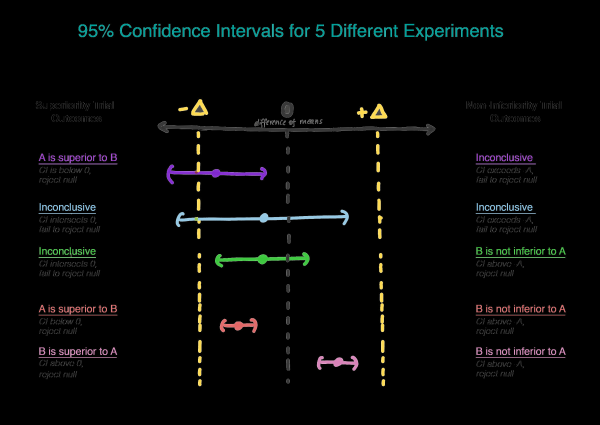
Choosing Δ
How should we choose Δ? The process of choosing Δ involves statistical justification and subject matter assessment. In the world of clinical research, there are regulatory guidelines indicating that delta should represent the smallest clinically significant difference—one that will matter in practice. Here is a quote from the European guidelines to help check yourself: 'If the difference has been chosen correctly, a confidence interval that is entirely between –∆ and 0... is still sufficient to demonstrate non-inferiority. If this result does not seem acceptable, it means that ∆ was not chosen appropriately.'
The delta should definitely not exceed the effect size of version A relative to the true control (placebo / no treatment), as this would imply that version B is worse than the true control while simultaneously demonstrating 'no less efficacy'. Assume that when version A was presented, there was a version 0 or the function did not exist at all (see Figure 3).
According to the results of the superiority hypothesis test, an effect size E was identified (i.e., presumably μ^A−μ^0=E). Now A is our new standard, and we want to ensure that B is not inferior to A. Another way to write μB−μA≤−Δ (the null hypothesis) is μB≤μA−Δ. If we assume that it is equal to or greater than E, then μB ≤ μA−E ≤ placebo. Now we see that our estimate for μB completely exceeds μA−E, thus completely refuting the null hypothesis and allowing us to conclude that B is not inferior to A, yet at the same time μB may be ≤ μ placebo, which is not what we want. (Figure 3).
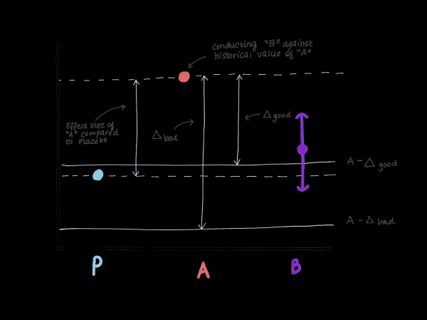
Figure 3. Demonstration of the risks of choosing a non-inferiority margin. If the margin is too large, one might conclude that B is not inferior to A, yet is indistinguishable from placebo. We would not want to switch to a treatment that is clearly less effective than placebo (A) for one that has the same efficacy as placebo.
Choosing α
Let’s move on to choosing α. The standard value of α = 0.05 can be used, but this is not entirely fair. For instance, when you purchase something online and use multiple discount codes simultaneously, which should not stack—it's just that the developer made a mistake, and you got away with it. According to the rules, the value of α should be half of the α used in the superiority hypothesis test, i.e., 0.05 / 2 = 0.025.
Sample Size
How do you estimate the sample size? If you believe that the true difference in means between A and B is 0, then the sample size calculation would be the same as for testing the superiority hypothesis, except that you replace the effect size with the non-inferiority margin, provided that you use αnon-inferiority = 1/2 αsuperiority (αnon-inferiority=1/2αsuperiority). If you have reason to believe that variant B might be slightly worse than variant A, but you want to prove that it is not worse by more than Δ, then you are in luck! In fact, this reduces your sample size because it is easier to demonstrate that B is worse than A if you actually believe it is slightly worse and not equivalent.
Example with a decision
Suppose you want to switch to version B on the condition that it is not worse than version A by more than 0.1 points on a 5-point customer satisfaction scale... Let's approach this task using the superiority hypothesis.
To test the superiority hypothesis, we would calculate the sample size as follows:
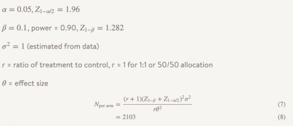
That is, if you have 2103 observations in your group, you can be 90% confident that you will detect an effect size of 0.10 or greater. But if the value of 0.10 is too large for you, it may not be worth testing the superiority hypothesis for it. Perhaps for reliability, you decide to conduct a study for a smaller effect size, for example, 0.05. In this case, you would need 8407 observations, which means the sample size increases nearly 4 times. But what if we stick to our original sample size but increase the power to 0.99, so we are not unsure if we get a positive result? In that case, n for one group would be 3676, which is already better, but it increases the sample size by more than 50%. And as a result, we still just won't be able to refute the null hypothesis, not to get an answer to our question.
What if instead we test the hypothesis of non-inferiority?

The sample size will be calculated using the same formula except for the denominator.
The differences from the formula used for testing the superiority hypothesis are as follows:
— Z1−α/2 is replaced with Z1−α, but if you do everything by the rules, you replace α = 0.05 with α = 0.025, meaning that it's the same number (1.96)
— (μB−μA) appears in the denominator
— θ (effect size) is replaced with Δ (non-inferiority margin)
If we assume that µB = µA, then (µB − µA) = 0 and the calculation of sample size for the non-inferiority limit is exactly what we would obtain when calculating superiority for an effect size of 0.1, great! We can conduct a study of the same scale with different hypotheses and a different approach to conclusions, and we will get the answer to the question we really want to answer.
Now let’s assume that we actually do not believe that µB = µA and
we think that µB is slightly worse, perhaps by 0.01 units. This increases our denominator, reducing the sample size for the group to 1737.
What happens if version B is actually better than version A? We reject the null hypothesis that B is worse than A by more than Δ and accept the alternative hypothesis that B, if worse, is not worse than Δ, and may be better. Try to incorporate this conclusion into a cross-functional presentation and see what comes of it (seriously, give it a try). In situations where we need to orient to perspective, no one wants to agree to 'not worse than Δ and possibly better.'
In this case, we can conduct a study that is very briefly called 'hypothesis testing of whether one option outperforms or underperforms another.' It uses two sets of hypotheses:
The first set (the same as in testing for non-inferiority):

The second set (the same as in testing for superiority):

We only test the second hypothesis if the first is rejected. Through sequential testing, we maintain the overall type I error rate (α). In practice, this can be achieved by constructing a 95% confidence interval for the difference between the means and testing to see if the entire interval exceeds -Δ. If the interval does not exceed -Δ, we cannot reject the null hypothesis and stop. If the entire interval does exceed -Δ, we will continue and check if the interval contains 0.
There is another type of research that we have not discussed – equivalence studies.
This type of research can be replaced by studies aimed at testing the hypothesis of non-inferiority and vice versa, but they have a significant difference. The hypothesis test for non-inferiority aims to demonstrate that option B is at least as good as A. In contrast, an equivalence study aims to show that option B is at least as good as A, and option A is at least as good as B, which is more complex. Essentially, we are trying to determine whether the entire confidence interval for the difference in means lies between −Δ and Δ. Such studies require a larger sample size and are conducted less frequently. Therefore, the next time you conduct a study where your main goal is to ensure that the new version is not worse, do not settle for “failing to reject the null hypothesis.” If you want to test a truly important hypothesis, consider various options.
Source: habr.com
