How to Read This Article: I apologize for the lengthy and chaotic nature of the text. To save your time, I begin each chapter with an introduction 'What I Learned,' summarizing the essence of the chapter in one or two sentences.

"Just Show Me the Solution!" If you simply want to see what I arrived at, jump to the chapter 'Becoming More Resourceful,' but I believe it's more interesting and beneficial to read about the failures.

Recently, I was tasked with setting up a process for handling a large volume of DNA sequence data (technically, this is SNP chip data). We needed to quickly obtain data on a specified genetic location (called an SNP) for further modeling and other tasks. Using R and AWK, I managed to clean and organize the data organically, significantly speeding up query processing. This was not easy for me and required numerous iterations. This article will help you avoid some of my mistakes and demonstrate what I ultimately achieved.

For starters, some introductory explanations.

Data

Our university's genetic information processing center provided us with data in the form of a 25 TB TSV file. I received it split into 5 packages, compressed with Gzip, each containing about 240 four-gigabyte files. Each row contained data for one SNP of one individual. In total, data for about 2.5 million SNPs and ~60,000 individuals were transmitted. Besides SNP information, the files contained numerous columns of numbers reflecting various characteristics, such as read intensity, allele frequency, etc. There were about 30 columns with unique values.

The goal

As in any data management project, the most important task was to determine how the data would be used. In this case, we will primarily be selecting models and workflows for SNP based on the SNP. That is, we will only need data for one SNP at a time. I had to learn to extract all records related to one of the 2.5 million SNPs as simply, quickly, and cheaply as possible.

How Not to Do This

Let me quote a fitting cliché:

I have not failed a thousand times; I have merely discovered a thousand ways not to parse a bunch of data into a query-friendly format.

First attempt

What I Learned: there is no cheap way to parse 25 TB at once.

After taking the course 'Advanced Methods for Processing Big Data' at Vanderbilt University, I was confident it would be straightforward. It would probably take an hour or two to set up a Hive server to run through all the data and report back the results. Since our data is stored in AWS S3, I utilized the service Athena, which allows Hive SQL queries to be applied to S3 data. There’s no need to set up or launch a Hive cluster, and you only pay for the data you query.

After I showed Athena my data and its format, I ran a few tests with such queries:

select * from intensityData limit 10;

And quickly received well-structured results. Done.

Until we tried to use the data in practice...

I was asked to extract all the SNP information to test it on a model. I ran the query:

select * from intensityData 
where snp = 'rs123456';

...and waited. After eight minutes and more than 4 TB of requested data, I got the result. Athena charges based on the volume of data found, at $5 per terabyte. So this single query cost $20 and took eight minutes to wait. To run the model on all the data, it would have taken 38 years and cost $50 million. Obviously, this wasn't feasible for us.

We needed to use Parquet...

What I Learned: be careful with the size and organization of your Parquet files.

Initially, I tried to rectify the situation by converting all TSV files into Parquet files. They are convenient for working with large datasets because information is stored in columnar format: each column resides in its own memory/disk segment, unlike text files where rows contain elements of each column. And if you need to find something, you only need to read the necessary column. Furthermore, each file contains a range of values in each column, so if the sought value is not within the column's range, Spark won't waste time scanning the entire file.

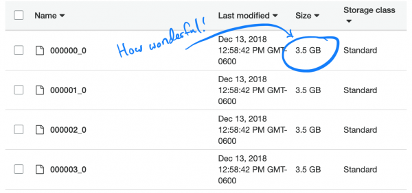
I ran a simple task AWS Glue to convert our TSV to Parquet and uploaded new files to Athena. It took about 5 hours. But when I ran the query, it took roughly the same amount of time and a little less money. The issue is that Spark, in an attempt to optimize the task, simply unpacked one TSV chunk and placed it in its own Parquet chunk. And since each chunk was quite large and contained full records for many individuals, every file held all SNPs, so Spark had to open all files to extract the necessary information.

Interestingly, the default (and recommended) compression type in Parquet — snappy — is not splitable. Therefore, each executor got stuck on the task of unpacking and loading the full dataset of 3.5 GB.

Let’s dive into the problem

What I Learned: sorting is difficult, especially when the data is distributed.

I thought I finally understood the essence of the problem. I just needed to sort the data by the SNP column, not by individuals. Then there would be several SNPs stored in a separate data chunk, and then the 'smart' Parquet function 'open only if the value is within range' would manifest itself beautifully. Unfortunately, sorting billions of rows scattered across the cluster turned out to be a challenging task.

Me taking algorithms class in college: “Ugh, no one cares about the computational complexity of all these sorting algorithms”

Me trying to sort on a column in a 20TB #spark table: “Why is this taking so long?” #DataScience struggles.

— Nick Strayer (@NicholasStrayer) March 11, 2019

AWS certainly doesn't want to refund for the reason of 'I’m a scatterbrained student.' After I started the sort on Amazon Glue, it ran for 2 days and failed.

What about partitioning?

What I Learned: partitions in Spark need to be balanced.

Then I had the idea to partition data by chromosomes. There are 23 of them (and a few more if you consider mitochondrial DNA and unmapped regions).
This will allow breaking the data into smaller portions. If I simply add one line to the Spark export function in the Glue script partition_by = "chr", then the data should be distributed into buckets.

The genome consists of numerous fragments called chromosomes.

Unfortunately, it didn't work. The chromosomes vary in size, which means they contain different amounts of information. This implies that the tasks Spark was sending to the workers were not balanced and were running slowly, as some nodes finished earlier and were idle. However, the tasks were completed. But when querying a single SNP, the imbalance caused problems again. The processing cost for SNP in larger chromosomes (i.e., from where we want to obtain data) only decreased by about 10 times. That's a lot, but not enough.

What if we divide into even smaller partitions?

What I Learned: never attempt to create 2.5 million partitions.

I decided to go all out and partitioned each SNP. This ensured equal partition sizes. IT WAS A BAD IDEA. I used Glue and added an innocent line partition_by = 'snp'. The job started and began executing. A day later I checked and saw that nothing had been written to S3 yet, so I killed the job. It seems Glue was writing intermediate files to a hidden location in S3, and there were many files, possibly a couple of million. As a result, my mistake cost over a thousand dollars and did not please my mentor.

Partitioning + sorting

What I Learned: sorting is still difficult, as is configuring Spark.

The last attempt at partitioning involved partitioning the chromosomes and then sorting each partition. In theory, this would speed up each query since the desired SNP data should be within a few Parquet chunks in the given range. Unfortunately, sorting even partitioned data turned out to be a challenging task. As a result, I moved to EMR for a custom cluster and used eight powerful instances (C5.4xl) and Sparklyr to create a more flexible workflow…

# Sparklyr snippet to partition by chr and sort w/in partition
# Join the raw data with the snp bins
raw_data
  group_by(chr) %>%
  arrange(Position) %>% 
  Spark_write_Parquet(
    path = DUMP_LOC,
    mode = 'overwrite',
    partition_by = c('chr')
  )

…however, the task still remained uncompleted. I tried various configurations: increasing memory allocation for each request executor, using nodes with larger memory, applying broadcasting variables, but each time it turned out to be a half measure, and gradually the executors began to fail until everything stopped.

Update: so it begins. pic.twitter.com/agY4GU2ru5

— Nick Strayer (@NicholasStrayer) May 15, 2019

I’m becoming more inventive

What I Learned: sometimes special data requires special solutions.

Each SNP has a position value. This number corresponds to the count of bases along its chromosome. It's a good and natural way to organize our data. Initially, I wanted to partition by regions of each chromosome. For example, positions 1-2000, 2001-4000, and so on. But the issue is that SNPs are unevenly distributed across chromosomes, thus the group sizes will vary significantly.

As a result, I arrived at a categorization (rank) of positions. Using the already uploaded data, I ran a query to obtain a list of unique SNPs, their positions, and chromosomes. Then I sorted the data within each chromosome and grouped the SNPs into bins of a specified size. Let's say, 1000 SNPs. This gave me the relationship of SNPs to bin-in-chromosome.

In the end, I created bins of 75 SNPs, which I will explain below.

snp_to_bin % 
  group_by(chr) %>% 
  arrange(position) %>% 
  mutate(
    rank = 1:n()
    bin = floor(rank/snps_per_bin)
  ) %>% 
  ungroup()

First attempt with Spark

What I Learned: combining in Spark works quickly, but partitioning is still costly.

I wanted to read this small (2.5 million rows) data frame into Spark, merge it with the raw data, and then partition it by the newly added column. bin.

# Join the raw data with the snp bins
data_w_bin <- raw_data %>%
  left_join(sdf_broadcast(snp_to_bin), by ='snp_name') %>%
  group_by(chr_bin) %>%
  arrange(Position) %>% 
  Spark_write_Parquet(
    path = DUMP_LOC,
    mode = 'overwrite',
    partition_by = c('chr_bin')
  )

I used sdf_broadcast(), so Spark knows it should send the data frame to all nodes. This is useful if the data is small and needed for all tasks. Otherwise, Spark tries to be smart and distributes data as needed, which can cause slowdowns.

And again my idea didn't work: tasks worked for a while, completed the merge, and then, like the partitioning executors that were launched, started to crash.

Adding AWK

What I Learned: don't sleep when you are taught the basics. Surely someone has solved your problem back in the 1980s.

Up until this point, the reason for all my failures with Spark was the mixing of data in the cluster. Perhaps the situation can be improved with preprocessing. I decided to try splitting the raw text data into chromosome columns, hoping to provide Spark with "pre-partitioned" data.

I searched on StackOverflow how to split by column values and found such a wonderful answer. With AWK, you can split a text file by column values by executing a script instead of sending the results to stdout.

As a trial, I wrote a Bash script. I downloaded one of the packed TSV files, then unpacked it using gzip and sent it to awk.

gzip -dc path/to/chunk/file.gz |
awk -F 't' 
'{print $1",..."$30">"chunked/"$chr"_chr"$15".csv"}'

It worked!

Filling the cores

What I Learned: gnu parallel is a magical thing; everyone should use it.

The splitting was quite slow, and when I ran htop, to check the utilization of a powerful (and expensive) EC2 instance, I found that I was only using one core and about 200 MB of memory. To solve the problem and avoid losing a lot of money, I needed to figure out how to parallelize the work. Fortunately, in the absolutely amazing book Data Science at the Command Line by Jeroen Janssens, I found a chapter dedicated to parallelization. From it, I learned about gnu parallel, a very flexible method for implementing multithreading in Unix.

When I started splitting using the new process, everything was great, but there remained a bottleneck — downloading S3 objects to disk was not very fast and not fully parallelized. To fix this, I did the following:

1. I figured out that you can directly implement the S3 download stage in the pipeline, completely eliminating the intermediate storage on disk. This means I can avoid writing raw data to disk and use even smaller, and thus cheaper, storage on AWS.
2. The command aws configure set default.s3.max_concurrent_requests 50 significantly increased the number of threads used by AWS CLI (by default, it's 10).
3. I switched to a network-optimized EC2 instance, with the letter n in its name. I found that the loss of computing power when using n-instances is more than compensated for by the increased upload speed. For most tasks, I used c5n.4xl.
4. I changed gzip to pigz, it's a gzip tool that does cool things for parallelizing an originally non-parallelizable file unpacking task (this helped the least).

# Let S3 use as many threads as it wants
aws configure set default.s3.max_concurrent_requests 50

for chunk_file in $(aws s3 ls $DATA_LOC | awk '{print $4}' | grep 'chr'$DESIRED_CHR'.csv') ; do

        aws s3 cp s3://$batch_loc$chunk_file - |
        pigz -dc |
        parallel --block 100M --pipe  
        "awk -F 't' '{print $1",..."$30">"chunked/{#}_chr"$15".csv"}'"

       # Combine all the parallel process chunks to single files
        ls chunked/ |
        cut -d '_' -f 2 |
        sort -u |
        parallel 'cat chunked/*_{} | sort -k5 -n -S 80% -t, | aws s3 cp - '$s3_dest'/batch_'$batch_num'_{}'
        
         # Clean up intermediate data
       rm chunked/*
done

These steps are combined with each other to make everything work very quickly. Thanks to the increased download speed and the elimination of writing to disk, I was now able to process a 5-terabyte batch in just a few hours.

There's nothing sweeter than seeing all the cores you're paying for on AWS being used. Thanks to gnu-parallel, I can unzip and split a 19GB CSV just as fast as I can download it. I couldn't even get Spark to run this. #DataScience #Linux pic.twitter.com/Nqyba2zqEk

— Nick Strayer (@NicholasStrayer) May 17, 2019

This tweet was supposed to mention 'TSV'. Unfortunately.

Using re-parsed data

What I Learned: Spark loves uncompressed data and doesn't like to combine partitions.

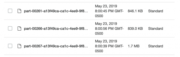
Now the data was in S3 in an uncompressed (read, delimited) and semi-ordered format, and I could return to Spark. I was in for a surprise: I still couldn't achieve the desired outcome! It was very difficult to tell Spark how the data was partitioned. And even when I did that, it turned out there were too many partitions (95K), and when I used coalesce to reduce the number to reasonable limits, it broke my partitioning. I'm sure it can be fixed, but after a couple of days of searching, I couldn't find a solution. In the end, I completed all tasks in Spark, although it took some time, and my split Parquet files were not very small (~200KB). However, the data was exactly where it needed to be.

Too small and inconsistent, wonderful!

Testing local Spark queries

What I Learned: Spark has too much overhead when solving simple tasks.

After loading the data in a thoughtful format, I was able to test the speed. I set up a script in R to run a local Spark server, then loaded the Spark data frame from the specified Parquet group storage (bin). I tried to load all the data, but I couldn't get Sparklyr to recognize the partitioning.

sc <- Spark_connect(master = "local")

desired_snp <- 'rs34771739'

# Start a timer
start_time <- Sys.time()

# Load the desired bin into Spark
intensity_data % 
  Spark_read_Parquet(
    name = 'intensity_data', 
    path = get_snp_location(desired_snp),
    memory = FALSE )

# Subset bin to snp and then collect to local
test_subset % 
  filter(SNP_Name == desired_snp) %>% 
  collect()

print(Sys.time() - start_time)

Execution took 29.415 seconds. Much better, but still not great for mass testing of anything. Also, I couldn't speed it up with caching because when I tried to cache the data frame in memory, Spark always crashed, even when I allocated more than 50GB of memory for a dataset that weighed less than 15.

Returning to AWK

What I Learned: associative arrays in AWK are very efficient.

I realized that I could achieve higher speeds. I remembered the wonderful AWK guide by Bruce Barnett I read about a cool feature called “associative arrays”. Essentially, these are key-value pairs, which for some reason were named differently in AWK, and that's probably why I hadn't really thought about them much. Roman Cheplyaka reminded me that the term “associative arrays” is much older than the term “key-value pair.” Even if you search for key-value in Google Ngram, you won’t find that term there; instead, you’ll find associative arrays! Moreover, “key-value pair” is most often associated with databases, so it makes much more sense to compare it to a hashmap. I realized that I could use these associative arrays to link my SNPs with the bin table and raw data without using Spark.

For this, I used a block in the AWK script BEGIN. This is a code fragment that executes before the first line of data is passed into the main body of the script.

join_data.awk
BEGIN {
  FS=",";
  batch_num=substr(chunk,7,1);
  chunk_id=substr(chunk,15,2);
  while(getline  "chunked/chr_"chr"_bin_"bin[$1]"_"batch_num"_"chunk_id".csv"
}

The command while(getline...) loaded all the rows from the CSV group (bin), setting the first column (SNP name) as the key for the associative array bin and the second value (group) as the value. Then in the block { }, which executes for all rows of the main file, each row is sent to an output file that gets a unique name based on its group (bin): ..._bin_"bin[$1]"_....

Variables batch_num and chunk_id corresponded to the data provided by the pipeline, which helped avoid a race condition, and each execution thread running in parallel, wrote to its own unique file.

Since I had scattered all raw data into folders by chromosomes left over from my previous experiment with AWK, I could now write another Bash script to process one chromosome at a time and deliver more deeply partitioned data to S3.

DESIRED_CHR='13'

# Download chromosome data from s3 and split into bins
aws s3 ls $DATA_LOC |
awk '{print $4}' |
grep 'chr'$DESIRED_CHR'.csv' |
parallel "echo 'reading {}'; aws s3 cp "$DATA_LOC"{} - | awk -v chr=""$DESIRED_CHR"" -v chunk="{}" -f split_on_chr_bin.awk"

# Combine all the parallel process chunks to single files and upload to rds using R
ls chunked/ |
cut -d '_' -f 4 |
sort -u |
parallel "echo 'zipping bin {}'; cat chunked/*_bin_{}_*.csv | ./upload_as_rds.R '$S3_DEST'/chr_'$DESIRED_CHR'_bin_{}.rds"
rm chunked/*

The script has two sections in parallel.

In the first section, data is read from all files containing information about the necessary chromosome, and then this data is distributed across threads that sort the files into appropriate groups (bins). To avoid race conditions when multiple threads write to the same file, AWK provides file names for writing data to different locations, for example, chr_10_bin_52_batch_2_aa.csv. As a result, many small files are created on disk (for this I used terabyte EBS volumes).

The pipeline from the second section in parallel processes the groups (bins) and merges their individual files into common CSVs with cat, and then sends them for export.

Translating into R?

What I Learned: you can access stdin and stdout from an R script, which means you can also use it in the pipeline.

In the Bash script, you might have noticed the following line: ...cat chunked/*_bin_{}_*.csv | ./upload_as_rds.R.... It translates all concatenated files of the group (bin) into the R script mentioned below. {} is a special technique in parallel, which inserts any data sent to the specified stream directly into the command itself. The option {#} provides a unique execution thread ID, while {%} is the job slot number (it repeats but never simultaneously). A list of all options can be found in of the documentation.

#!/usr/bin/env Rscript
library(readr)
library(aws.s3)

# Read first command line argument
data_destination <- commandArgs(trailingOnly = TRUE)[1]

data_cols <- list(SNP_Name = 'c', ...)

s3saveRDS(
  read_csv(
        file("stdin"), 
        col_names = names(data_cols),
        col_types = data_cols 
    ),
  object = data_destination
)

When the variable file("stdin") is passed to readr::read_csv, the data translated into the R script is loaded into a frame, which is then saved in the form of .rds-file using aws.s3 is written directly to S3.

RDS is somewhat like a junior version of Parquet, without the complexities of a columnar store.

After completing the Bash script, I received a batch of .rds-files sitting in S3, allowing me to utilize efficient compression and built-in types.

Despite using the slow R, everything worked very quickly. It's no surprise that the R fragments responsible for reading and writing data are well optimized. After testing on a medium-sized chromosome, the task was completed on a C5n.4xl instance in about two hours.

S3 limitations

What I Learned: thanks to smart path implementations, S3 can handle many files.

I was concerned whether S3 could process the many files sent to it. I could give the file names meaning, but how would S3 search through them?

Folders in S3 are just for aesthetics; in reality, the system doesn't care about the symbol /. From the S3 FAQ page.

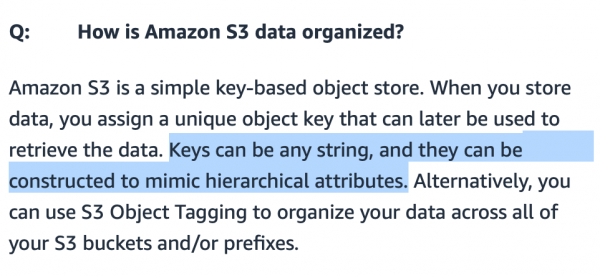
It seems that S3 represents the path to a specific file as a simple key in a sort of hash table or document-based database. A bucket can be considered a table, and files are the records in that table.

Since speed and efficiency are crucial for profitability on Amazon, it's no surprise that this 'key-as-file-path' system is brilliantly optimized. I tried to find a balance: to avoid making numerous get requests while ensuring that requests were fast. It turned out that having around 20,000 binary files was optimal. I think if optimization continues, speed could be improved (for instance, by creating a special bucket just for the data, thus reducing the size of the search table). But there wasn't enough time and budget for further experiments.

What about cross-compatibility?

What I learned: the main reason for wasting time is premature optimization of your storage method.

At this point, it’s crucial to ask yourself: 'Why use a proprietary file format?' The reason lies in the loading speed (compressed gzip CSV files took 7 times longer to load) and compatibility with our workflows. I might reconsider my decision if R can easily load Parquet (or Arrow) files without the overhead of Spark. Everyone in our lab uses R, and if I need to convert the data to another format, I still have the original text data, so I can simply rerun the pipeline.

Work Division

What I Learned: do not attempt to optimize tasks manually; let the computer do it.

I debugged the workflow on one chromosome; now I need to process all the other data.
I wanted to spin up a few EC2 instances for processing, but at the same time, I was concerned about getting a highly imbalanced load across different processing tasks (just as Spark suffered from unbalanced partitions). Furthermore, I was reluctant to spin up one instance for each chromosome because there’s a default limit of 10 instances for AWS accounts.

So, I decided to write a script in R to optimize the processing tasks.

First, I asked S3 to compute how much storage space each chromosome occupies.

library(aws.s3)
library(tidyverse)

chr_sizes % 
  mutate(Size = as.numeric(Size)) %>% 
  filter(Size != 0) %>% 
  mutate(
    # Extract chromosome from the file name 
    chr = str_extract(Key, 'chr.{1,4}.csv') %>%
             str_remove_all('chr|.csv')
  ) %>% 
  group_by(chr) %>% 
  summarise(total_size = sum(Size)/1e+9) # Divide to get value in GB



# A tibble: 27 x 2
   chr   total_size
         
 1 0           163.
 2 1           967.
 3 10          541.
 4 11          611.
 5 12          542.
 6 13          364.
 7 14          375.
 8 15          372.
 9 16          434.
10 17          443.
# … with 17 more rows

Then I wrote a function that takes the total size, randomizes the order of chromosomes, and divides them into groups. num_jobs and reports how the sizes of all processing jobs vary.

num_jobs <- 7
# How big would each job be if perfectly split?
job_size <- sum(chr_sizes$total_size)/7

shuffle_job %
    sample_frac() %>% 
    mutate(
      cum_size = cumsum(total_size),
      job_num = ceiling(cum_size/job_size)
    ) %>% 
    group_by(job_num) %>% 
    summarise(
      job_chrs = paste(chr, collapse = ','),
      total_job_size = sum(total_size)
    ) %>% 
    mutate(sd = sd(total_job_size)) %>% 
    nest(-sd)
}

shuffle_job(1)



# A tibble: 1 x 2
     sd data            
             
1  153.

Then I ran a thousand shuffles using purrr and selected the best one.

1:1000 %>% 
  map_df(shuffle_job) %>% 
  filter(sd == min(sd)) %>% 
  pull(data) %>% 
  pluck(1)

This way, I got a set of jobs that were very similar in size. Then, I just needed to wrap my previous Bash script in a large loop. for. It took about 10 minutes to write this optimization. And that’s much less than I would have spent on manually creating jobs in case of their imbalance. So I think I did well with this preliminary optimization.

for DESIRED_CHR in "16" "9" "7" "21" "MT"
do
# Code for processing a single chromosome
fi

Finally, I add a shutdown command:

sudo shutdown -h now

… and it worked! Using the AWS CLI, I launched instances and passed them the Bash scripts of their processing jobs through the user_data which executed and automatically shut down, so I didn't pay for excess compute power.

aws ec2 run-instances ...
--tag-specifications "ResourceType=instance,Tags=[{Key=Name,Value=<>}]" 
--user-data file://<>

Let's pack it up!

What I Learned: The API should be simple for ease and flexibility of use.

Finally, I got the data in the right place and format. I needed to simplify the process of using the data as much as possible, making it easier for my colleagues. I wanted to create a simple API for making requests. If in the future I decide to switch to .rds When it comes to Parquet files, this should be a problem for me, not for my colleagues. To address this, I decided to create an internal R package.

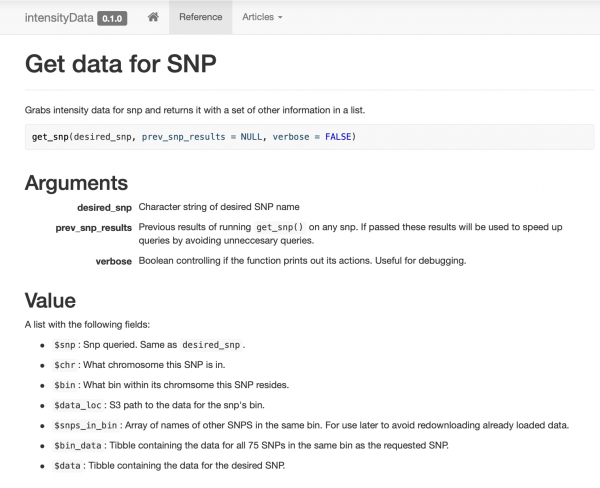
I assembled and documented a very simple package that contains just a few functions for accessing data built around the function get_snp. I also created a website for my colleagues pkgdown, so they could easily view examples and documentation.

Intelligent caching

What I Learned: if your data is well-prepared, caching will be easy!

Since one of the main workflows applied the same analysis model to the SNP package, I decided to use binning to my advantage. When passing SNP data, all information from the group (bin) is attached to the returned object. This means that old queries can (theoretically) speed up the processing of new requests.

# Part of get_snp()
...
  # Test if our current snp data has the desired snp.
  already_have_snp <- desired_snp %in% prev_snp_results$snps_in_bin

  if(!already_have_snp){
    # Grab info on the bin of the desired snp
    snp_results <- get_snp_bin(desired_snp)

    # Download the snp's bin data
    snp_results$bin_data <- aws.s3::s3readRDS(object = snp_results$data_loc)
  } else {
    # The previous snp data contained the right bin so just use it
    snp_results <- prev_snp_results
  }
...

While assembling the package, I ran many benchmarks to compare speed using different methods. I recommend not neglecting this, as the results can sometimes be surprising. For example, dplyr::filter turned out to be much faster than capturing rows using indexing-based filtering, and obtaining a single column from the filtered data frame worked much faster than applying indexing syntax.

Note that the object prev_snp_results contains the key snps_in_bin. This is an array of all unique SNPs in the group (bin), allowing for quick checks to see if data from a previous request already exists. It also simplifies looping through all SNPs in the group (bin) with the following code:

# Get bin-mates
snps_in_bin <- my_snp_results$snps_in_bin

for(current_snp in snps_in_bin){
  my_snp_results <- get_snp(current_snp, my_snp_results)
  # Do something with results 
}

Results

Now we can (and have seriously started) running models and scenarios that were previously unavailable to us. The best part is that my lab colleagues don’t have to worry about any complexities. They just have a working function.

And although the package relieves them of the details, I tried to make the data format simple enough for them to understand in case I suddenly disappear tomorrow...

The speed has noticeably increased. We usually scan functionally significant fragments of the genome. We couldn’t do this before (it was too expensive), but now, thanks to the bin structure and caching, a request for a single SNP takes on average less than 0.1 seconds, and the data usage is so low that the costs for S3 are negligible.

Recently I was put in charge of managing over 25 TB of raw genotyping data for my lab. When I started, using Spark took 8 minutes and cost $20 to query a SNP. After using AWK + #rstats to process, it now takes less than a tenth of a second and costs $0.00001. My personal #BigData win. pic.twitter.com/ANOXVGrmkk

— Nick Strayer (@NicholasStrayer) May 30, 2019

Conclusion

This article is not a guide at all. The solution turned out to be individual and almost certainly not optimal. Rather, it's a story about a journey. I want others to understand that such solutions don't come fully formed; they are the result of trials and errors. Furthermore, if you are looking for a data analysis specialist, keep in mind that effective use of these tools requires experience, and experience costs money. I am fortunate to have had the funds to pay for it, but many others who might do the same job better than I could will never have that opportunity due to lack of money even for a try.

Tools for big data are universal. If you have time, you can almost certainly write a faster solution by applying 'smart' data cleaning, storage, and extraction methods. Ultimately, it all comes down to a cost-benefit analysis.

What I've learned:

• there's no cheap way to parse 25 TB at once;
• be careful with the size of your Parquet files and their organization;
• partitions in Spark should be balanced;
• never attempt to create 2.5 million partitions;
• sorting is still difficult, just like tuning Spark;
• sometimes specific data requires specific solutions;
• joining in Spark works quickly, but partitioning still costs a lot;
• don't sleep when you're being taught the basics; surely someone resolved your problem back in the 1980s;
• gnu parallel — it’s a magical thing, everyone should use it;
• Spark loves uncompressed data and dislikes combining partitions;
• there’s too much overhead in Spark when dealing with simple tasks;
• associative arrays in AWK are very efficient;
• you can access stdin and stdout from R scripts, meaning you can also use it in the pipeline;
• thanks to smart implementation, S3 paths can handle many files;
• the main reason for wasting time is premature optimization of your storage method;
• don't try to optimize tasks manually; let the computer do it;
• the API should be simple for the sake of simplicity and flexibility in use;
• if your data is well prepared, caching will be easy!

Source: habr.com