The book "Kafka Streams in Action: Applications and Microservices for Real-Time Processing"

Hello, Habr readers! This book is suitable for any developer who wants to understand stream processing. Understanding distributed programming will enhance your knowledge of Kafka and Kafka Streams. It would be beneficial to know the Kafka framework itself, but it is not mandatory: I will cover everything you need to know. Experienced Kafka developers, as well as newcomers, will learn how to create interesting stream processing applications using the Kafka Streams library through this book. Java developers at intermediate and advanced levels, already familiar with concepts like serialization, will learn to leverage their skills for building Kafka Streams applications. The book's source code is written in Java 8 and extensively uses Java 8 lambda expression syntax, so being able to work with lambda functions (even in another programming language) will be useful.

Excerpt. 5.3. Aggregation and Window Operations

In this section, we will move on to exploring the most promising parts of Kafka Streams. So far, we have covered the following aspects of Kafka Streams:

• creating processing topologies;
• using state in streaming applications;
• performing data stream joins;
• the differences between event streams (KStream) and update streams (KTable).

In the next examples, we will bring all these elements together. Additionally, you will get acquainted with window operations — another remarkable feature of streaming applications. Our first example will be simple aggregation.

5.3.1. Aggregating Sales Volumes of Stocks by Industry

Aggregation and grouping are essential tools when working with streaming data. Analyzing individual records as they arrive is often insufficient. To extract additional information from the data, grouping and combining it is necessary.

In this example, you will don the role of an intraday trader who needs to track the sales volumes of stocks from companies in several industries. Specifically, you are interested in the five companies with the highest sales volumes in each industry.

For such aggregation, several steps will be required to transform the data into the desired format (speaking in general terms).

1. Create a source based on a topic that publishes raw information about stock trading. We have to map the StockTransaction object to the ShareVolume object. The StockTransaction object contains sales metadata, while we only need data on the number of shares sold.
2. Group the ShareVolume data by stock symbols. After grouping by symbols, we can reduce this data to intermediate sums of stock sales volumes. It is worth noting that the KStream.groupBy method returns an instance of KGroupedStream. An instance of KTable can be obtained by calling the reduce method on KGroupedStream.

What is the KGroupedStream interface?

The KStream.groupBy and KStream.groupByKey methods return an instance of KGroupedStream. KGroupedStream is an intermediate representation of the event stream after grouping by keys. It is not intended for direct manipulation. Instead, KGroupedStream is used for aggregation operations, the result of which is always a KTable. Since aggregation operations result in a KTable and utilize state storage, not all updates may be sent further down the pipeline.

The KTable.groupBy method returns an analogous KGroupedTable—an intermediate representation of the update stream regrouped by key.

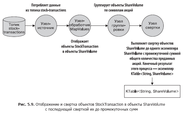
Let's take a short break and look at Fig. 5.9, which shows what we have achieved. This topology should already be familiar to you.

Now let’s look at the code for this topology (which can be found in the file src/main/java/bbejeck/chapter_5/AggregationsAndReducingExample.java) (Listing 5.2).

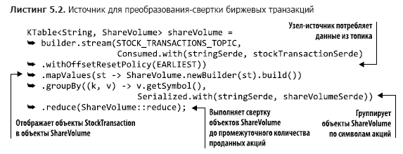
The provided code is concise and carries out a significant amount of actions in just a few lines. In the first parameter of the builder.stream method, you may notice something new to you: the value of the enumerated type AutoOffsetReset.EARLIEST (there is also LATEST), set using the Consumed.withOffsetResetPolicy method. This enumerated type allows you to specify the offset reset strategy for each KStream or KTable, taking priority over the offset reset parameter from the configuration.

GroupByKey and GroupBy

In the KStream interface, there are two methods for grouping records: GroupByKey and GroupBy. Both return a KGroupedTable, so you may have a reasonable question: what is the difference between them and when should each be used?

The GroupByKey method is applied when the keys in KStream are already populated. Importantly, the 'requires repartitioning' flag has never been set.

The GroupBy method assumes that you've changed the keys for grouping, so the repartitioning flag is set to true. Executing joins, aggregations, and so forth after the GroupBy method will automatically trigger repartitioning.
Summary: you should use GroupByKey whenever possible instead of GroupBy.

What the mapValues and groupBy methods do is clear, so let's take a look at the sum() method (which can be found in the file src/main/java/bbejeck/model/ShareVolume.java) (listing 5.3).

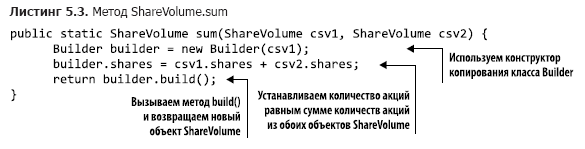
The ShareVolume.sum method returns the intermediate sum of share sales volume, and the result of the entire calculation chain is an object KTable. Now you understand the role of KTable. When ShareVolume objects arrive, the latest relevant update is stored in the corresponding KTable object. It's important to remember that all updates are reflected in the previous shareVolumeKTable, but not all are sent further.

Next, we use this KTable to perform aggregation (based on the number of shares sold) to obtain the top five companies with the highest share sales volume in each industry. Our actions here will be similar to those taken during the first aggregation.

1. Perform another groupBy operation to group individual ShareVolume objects by industry.
2. Start summing ShareVolume objects. This time, the aggregation object is a fixed-size priority queue. Only the top five companies with the highest volume of sold shares are kept in this fixed-size queue.
3. Map the queues from the previous step to a string value and return the five best-selling companies by share volume across industries.
4. Write the results as a string to the topic.

Figure 5.10 shows the graph of the data flow topology. As you can see, the second processing loop is quite simple.

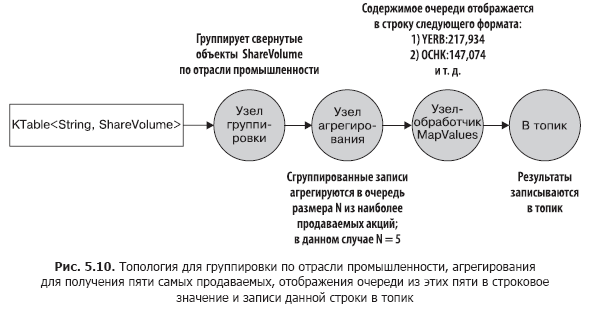
Now that you have a clear understanding of the structure of this second processing loop, you can refer to its source code (you will find it in the file src/main/java/bbejeck/chapter_5/AggregationsAndReducingExample.java) (listing 5.4).

In this initializer, there is a variable fixedQueue. This is a user-defined object—a wrapper for java.util.TreeSet—that is used to track the top N results in descending order of the number of shares sold.

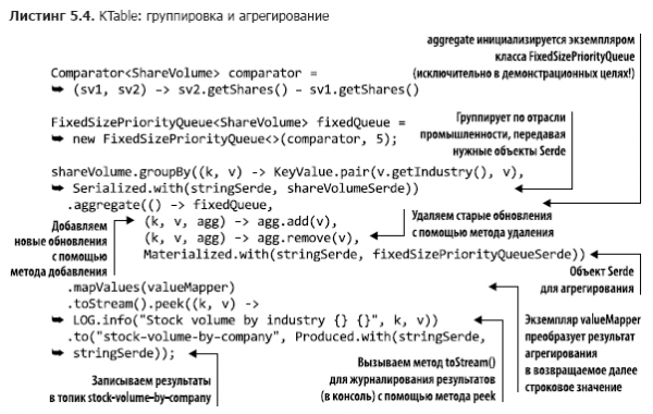
You have already encountered the groupBy and mapValues calls, so we won't dwell on them (we call the KTable.toStream method, as the KTable.print method is considered deprecated). However, you haven't seen the KTable version of the aggregate() method yet, so we'll spend some time discussing it.

As you recall, KTable distinguishes that records with the same keys are considered updates. KTable replaces the old record with a new one. Aggregation occurs similarly: the latest records with the same key are aggregated. When a record arrives, it is added to an instance of the FixedSizePriorityQueue using the aggregator (the second parameter in the aggregate method call), but if there is already another record with the same key, the old record is removed using the subtractor (the third parameter in the aggregate method call).

This means that our aggregator, FixedSizePriorityQueue, does not aggregate all values with one key but instead maintains a sliding sum of the quantities of the top N best-selling stock types. Each incoming record contains the total number of shares sold so far. KTable will provide you with information about which companies' shares are currently selling the most, and sliding aggregation of each update is not required.

We have learned to do two important things:

• group values in KTable by a common key;
• perform useful operations on these grouped values, such as folding and aggregation.

The ability to perform these operations is crucial for understanding the meaning of the data flowing through the Kafka Streams application and determining what information it conveys.

We have also brought together some key concepts discussed earlier in this book. In Chapter 4, we talked about the importance of resilient, local state for streaming applications. The first example from this chapter demonstrated why local state is so crucial—it allows tracking what information you have already seen. Local access helps avoid network delays, making the application more efficient and resilient to errors.

When performing any aggregation or folding operation, it is necessary to specify the name of the state store. Aggregation and folding operations return an instance of KTable, and KTable uses the state store to replace old results with new ones. As you have seen, not all updates are sent down the pipeline, which is important since aggregation operations are meant to yield final information. Without applying local state, KTable will send all results of aggregation and folding downstream.

Next, we will look at executing operations like aggregation over a specific period—so-called windowing operations.

5.3.2. Windowing Operations

In the previous section, we introduced 'sliding' aggregation and folding. The application performed continuous folding of stock sales volume followed by aggregation of the five best-selling stocks on the exchange.

Sometimes such continuous aggregation and folding of results are necessary. Other times, operations need to be performed only over a specified interval. For example, to calculate how many stock trades were conducted for a specific company in the last 10 minutes. Or how many users clicked on a new ad banner in the last 15 minutes. The application can perform these operations repeatedly, but with results pertaining only to the specified time intervals (time windows).

Counting stock transactions by buyer

In the next example, we will focus on tracking stock transactions for several traders—either large organizations or savvy solo investors.

There are two possible reasons for such tracking. One is the need to know what market leaders are buying and selling. If these major players and savvy investors see emerging opportunities, it makes sense to follow their strategy. The second reason is the desire to detect any signs of illegal transactions using insider information. For this, you will need to analyze the correlation of large spikes in sales with significant press releases.

This tracking consists of several stages, such as:

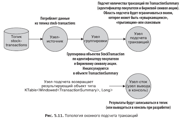
• creating a stream to read from the topic stock-transactions;
• grouping incoming records by buyer ID and stock ticker. The groupBy method returns an instance of the KGroupedStream class;
• returning data through KGroupedStream.windowedBy, limiting the data stream by a time window, allowing for windowed aggregation. Depending on the type of window, either TimeWindowedKStream or SessionWindowedKStream is returned;
• counting transactions for aggregation purposes. The windowed data stream defines whether a specific record is counted in this process;
• writing results to a topic or outputting them to the console during development.

The topology of this application is simple, but a visual representation would be helpful. Let's look at Fig. 5.11.

Next, we will discuss the functionality of window operations and the corresponding code.

Types of Windows

In Kafka Streams, there are three types of windows:

• session;
• tumbling;
• sliding/hopping.

Which one to choose depends on business requirements. Tumbling and hopping windows are time-limited, whereas session constraints are related to user actions—the duration of sessions is defined solely by how actively the user behaves. The key thing to remember is that all types of windows are based on the timestamps of records, not on system time.

Next, we will implement our topology with each of the window types. The complete code will be provided only in the first example; for the other window types, nothing will change except for the type of window operation.

Session Windows

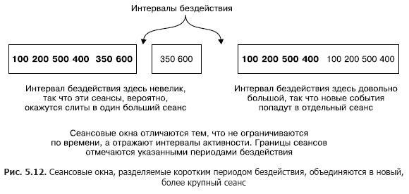
Session windows differ significantly from all other types of windows. They are limited not so much by time as by user activity (or the activity of the entity you wish to track). Session windows are delineated by periods of inactivity.

Figure 5.12 illustrates the concept of session windows. A shorter session will merge with the session to its left. The session to the right will be separate, as it follows a prolonged period of inactivity. Session windows are based on user actions but utilize date/time stamps from records to determine which session a record belongs to.

Using session windows to track stock market transactions

We will use session windows to capture information about stock market transactions. The implementation of session windows is shown in Listing 5.5 (which can be found in the file src/main/java/bbejeck/chapter_5/CountingWindowingAndKTableJoinExample.java).

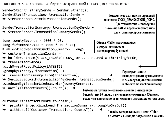
Most operations in this topology you have already encountered, so there is no need to discuss them here again. However, there are also a few new elements that we will discuss now.

In any groupBy operation, some form of aggregation operation (aggregation, folding, or counting) is usually performed. You can either perform cumulative aggregation with a running total or windowed aggregation, where records are taken into account within a specified time window.

The code from Listing 5.5 counts the number of transactions within session windows. In Fig. 5.13, these actions are analyzed step by step.

By calling windowedBy(SessionWindows.with(twentySeconds).until(fifteenMinutes)), we create a session window with an inactivity interval of 20 seconds and a retention interval of 15 minutes. The 20-second inactivity interval means that the application will include any record that arrives within 20 seconds of the end or start of the current session into the current (active) session.

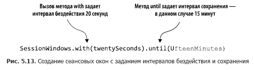
Next, we specify the aggregation operation to be performed in the session window — in this case, count. If an incoming record exceeds the inactivity interval (from either side of the timestamp), the application creates a new session. The retention interval means maintaining a session for a certain period and allows late data that falls outside the session's inactivity period but can still be appended. Furthermore, the start and end of the new session obtained from merging correspond to the earliest and latest timestamps.

Let's consider several records from the count method to see how sessions work (Table 5.1).

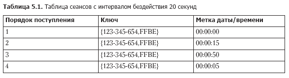
When records arrive, we look for existing sessions with the same key, where the end time is less than the current timestamp — the inactivity interval, and start time is greater than the current timestamp plus the inactivity interval. Based on this, four records from Table 5.1 merge into a single session as follows.

1. The first record is Record 1, so the start time equals the end time and is equal to 00:00:00.

2. Next comes Record 2, and we look for sessions ending no earlier than 23:59:55 and starting no later than 00:00:35. We find Record 1 and merge Sessions 1 and 2. We take the start time of Session 1 (earlier) and the end time of Session 2 (later), so our new session starts at 00:00:00 and ends at 00:00:15.

3. Record 3 arrives, we look for sessions between 00:00:30 and 00:01:10 and find none. We add a second session for the key 123-345-654,FFBE, starting and ending at 00:00:50.

4. Record 4 arrives, and we search for sessions between 23:59:45 and 00:00:25. This time both sessions — 1 and 2 — are found. All three sessions merge into one, with a start time of 00:00:00 and an end time of 00:00:15.

From what has been discussed in this section, the following important nuances should be remembered:

• sessions are not fixed-size windows. The duration of a session is determined by activity within a specified timeframe;
• timestamps in the data determine whether an event falls into an existing session or an inactivity interval.

Next, we will discuss the next type of windows — "tumbling" windows.

"Tumbling" windows

"Tumbling" windows capture events occurring within a specific time frame. Imagine you need to capture all stock transaction data for a company every 20 seconds, so you collect all events during this time. At the end of the 20-second interval, the window "tumbles" and moves on to a new 20-second observation window. Figure 5.14 illustrates this situation.

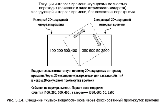
As you can see, all events that occurred in the last 20 seconds are included in the window. After this time period, a new window is created.

Listing 5.6 shows code demonstrating the use of "tumbling" windows to capture stock transactions every 20 seconds (it can be found in the file src/main/java/bbejeck/chapter_5/CountingWindowingAndKtableJoinExample.java).

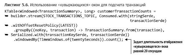
Thanks to this small change in the method call TimeWindows.of, a "tumbling" window can be used. In this example, there is no call to the until() method, which means the default retention period of 24 hours will be used.

Finally, it’s time to move on to the last type of window – "hopping" windows.

Sliding ("hopping") windows

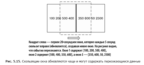
Sliding/"hopping" windows are similar to "tumbling" windows, but with a slight difference. Sliding windows do not wait for the end of the time interval before creating a new window to process recent events. They initiate new calculations after a waiting interval that is shorter than the window duration.

To illustrate the differences between "tumbling" and "hopping" windows, let’s return to the example of counting stock transactions. Our goal remains to count the number of transactions, but we do not want to wait for the entire time interval before updating the counter. Instead, we will update the counter at shorter intervals. For example, we will still count the number of transactions every 20 seconds, but update the counter every 5 seconds, as shown in Figure 5.15. This results in three overlapping windows of results.

Listing 5.7 contains the code for defining sliding windows (it can be found in the file src/main/java/bbejeck/chapter_5/CountingWindowingAndKtableJoinExample.java).

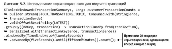
A "cascading" window can be transformed into a "jumping" window by adding a call to the advanceBy() method. In the given example, the retention period is set to 15 minutes.

In this section, you learned how to limit aggregation results using time windows. Specifically, remember the following three things from this section:

• the size of session windows is limited not by the time interval but by user activity;
• "cascading" windows provide insights into events within a specified time period;
• the duration of "jumping" windows is fixed, but they are frequently updated and may contain overlapping records across all windows.

Next, we will learn how to convert a KTable back into a KStream for joining.

5.3.3. Joining KStream and KTable objects

In Chapter 4, we discussed joining two KStream objects. Now we need to learn how to join a KTable and a KStream. This may be necessary for the simple reason that KStream is a stream of records, while KTable is a stream of record updates, but sometimes it may be needed to add additional context to the stream of records using updates from the KTable.

Let’s take data on the number of stock transactions and combine it with stock news based on corresponding industries. Here’s what needs to be done to achieve this given the existing code.

1. Convert the KTable object containing data on the number of stock transactions into a KStream by replacing the key with a key representing the industry corresponding to a given stock symbol.
2. Create a KTable object that reads data from the topic with stock news. This new KTable will be categorized by industry.
3. Join the news updates with the information on the number of stock transactions by industry.

Now let's look at how to implement this action plan.

Converting KTable to KStream

To convert KTable to KStream, you need to do the following.

1. Call the KTable.toStream() method.
2. Using the KStream.map method, replace the key with the name of the industry, and then extract a TransactionSummary object from the Windowed instance.

We will link these operations in a chain as follows (the code can be found in the file src/main/java/bbejeck/chapter_5/CountingWindowingAndKtableJoinExample.java) (listing 5.8).

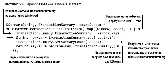
Since we are performing the KStream.map operation, the repartitioning for the returned instance of KStream is done automatically when it is used in a join.

We have completed the transformation process; now we need to create a KTable object to read stock market news.

Creating a KTable for stock market news

Fortunately, creating a KTable object requires only a single line of code (this code can be found in the file src/main/java/bbejeck/chapter_5/CountingWindowingAndKtableJoinExample.java) (listing 5.9).

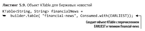
It is worth noting that no Serde objects need to be specified, as string Serdes are used in the settings. Additionally, by using the EARLIEST enumeration, the table is populated with records at the very beginning.

Now we can move on to the final step — the join.

Joining news updates with transaction count data

Creating the join is not difficult. We will use a left join in case there are no stock market news updates for the relevant industry (the required code can be found in the file src/main/java/bbejeck/chapter_5/CountingWindowingAndKtableJoinExample.java) (listing 5.10).

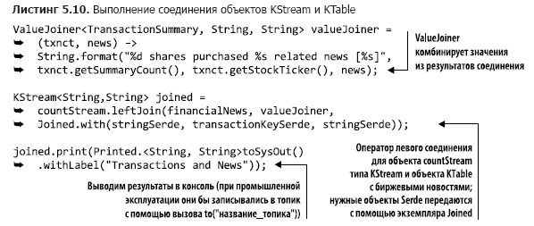
This leftJoin operator is quite simple. Unlike the joins from Chapter 4, the JoinWindow method is not used, since when performing a KStream-KTable join there is only one record for each key in the KTable. This join is not time-constrained: a record either exists in KTable or it does not. The main takeaway is that KTable objects can enrich KStream with less frequently updated reference data.

Now we will look at a more efficient way to enrich events from the KStream.

5.3.4. GlobalKTable Objects

As you have understood, there is a need to enrich event streams or add context to them. In Chapter 4, you saw joins between two KStream objects, and in the previous section — a join between KStream and KTable. In all these cases, it is necessary to repartition the data stream when mapping keys to a new type or value. Sometimes repartitioning is performed explicitly, while other times Kafka Streams does it automatically. Repartitioning is necessary since the keys have changed and records must end up in new partitions; otherwise, the join will not be possible (this was discussed in Chapter 4, in the section "Repartitioning Data" of subsection 4.2.4).

Resharding has its cost

Resharding requires expenses — additional resource costs for creating intermediate topics, storing duplicate data in yet another topic; it also means increased latency due to writing and reading from this topic. Furthermore, if you need to join on more than one aspect or dimension, you must chain the joins, project records with new keys, and then repeat the resharding process.

Joining with smaller datasets

In some cases, the volume of reference data to be joined is relatively small, so complete copies can fit locally on each node. For such situations, Kafka Streams provides the GlobalKTable class.

GlobalKTable instances are unique because the application replicates all data to each of the nodes. Since all nodes have all the data, there's no need to shard the event stream by the key of the reference data for it to be accessible to all shards. With GlobalKTable objects, you can also perform non-keyed joins. Let's return to one of the previous examples to demonstrate this capability.

Joining KStream objects with GlobalKTable objects

In subsection 5.3.2, we performed windowed aggregation of stock transactions by customers. The results of this aggregation looked something like this:

{customerId='074-09-3705', stockTicker='GUTM'}, 17
{customerId='037-34-5184', stockTicker='CORK'}, 16

Although these results met the set goal, it would be more convenient if the customer's name and full company name were also outputted. To add the buyer's name and company name, you can perform regular joins, but this would require two key mappings and resharding. Using GlobalKTable can help avoid the overhead of such operations.

To do this, we will use the countStream object from listing 5.11 (the corresponding code can be found in the file src/main/java/bbejeck/chapter_5/GlobalKTableExample.java), joining it with two GlobalKTable objects.

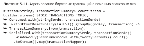
We discussed this earlier, so I won’t repeat myself. However, I would like to note that the code in the toStream().map function is abstracted into a function object for readability rather than using an embedded lambda expression.

The next step is the declaration of two instances of GlobalKTable (the provided code can be found in the file src/main/java/bbejeck/chapter_5/GlobalKTableExample.java) (listing 5.12).

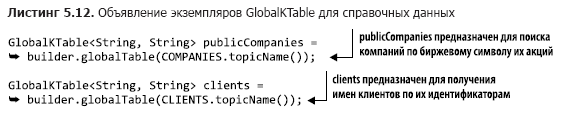
Note that topic names are described using enumerated types.

Now that we have prepared all the components, we just need to write the code for the join (which can be found in the file src/main/java/bbejeck/chapter_5/GlobalKTableExample.java) (listing 5.13).

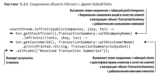
Although this code contains two joins, they are organized in a chain because none of their results are used separately. The results are output at the end of the entire operation.

When you run the join operation above, you will get results that look like this:

{customer='Barney, Smith' company="Exxon", transactions= 17}

The essence hasn't changed, but these results are clearer.

If you consider Chapter 4, you have already seen several types of joins in action. They are listed in Table 5.2. This table reflects the joining capabilities available for version 1.0.0 of Kafka Streams; in future releases, something may change.

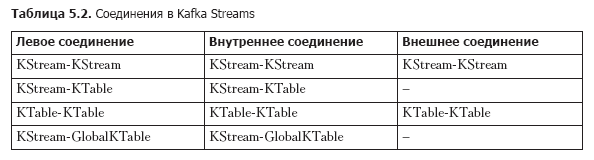
In conclusion, let me remind you of the main point: you can join event streams (KStream) and update streams (KTable) using local state. Additionally, if the size of the reference data is not too large, you can use the GlobalKTable object. GlobalKTable replicates all partitions to each node of the Kafka Streams application, providing access to all data regardless of which partition the key belongs to.

Next, we will look at a Kafka Streams feature that allows you to observe state changes without consuming data from the Kafka topic.

5.3.5. Queryable State

We have already performed several operations involving state and always output the results to the console (for development purposes) or wrote them to the topic (for production purposes). When writing results to a topic, you need to use a Kafka consumer to view them.

Reading data from these topics can be considered a form of materialized views. For our purposes, we can use the definition of a materialized view from Wikipedia: "...a physical database object that contains the results of a query. For example, it can be a local copy of remote data, or a subset of rows and/or columns of a table or results of a join, or a pivot table obtained through aggregation" (https://en.wikipedia.org/wiki/Materialized_view).

Kafka Streams also allows for interactive queries to state stores, enabling direct reading of these materialized views. It is important to note that requests to the state store are read-only operations. This means you do not need to worry about unintentionally making the state inconsistent during data processing by the application.

The ability to make direct queries to state stores is significant. It means you can create applications—dashboards—without needing to first retrieve data from the Kafka consumer. It also increases application efficiency since there is no need to rewrite data:

• due to the locality of the data, it can be accessed quickly;
• data duplication is eliminated as it is not written to external storage.

The main point I want you to remember is: you can execute queries directly on the state from the application. The capabilities this provides you cannot be overstated. Instead of consuming data from Kafka and storing records in a database for the application, you can query state stores with the same result. Direct queries to state stores mean less code (no consumer) and less software (no need for a database table to store results).

We have covered a considerable amount of information in this chapter, so we will pause our discussion on interactive queries to state stores for a moment. But don't worry: in Chapter 9, we will create a simple application — a dashboard with interactive queries. To demonstrate interactive queries and the ability to incorporate them into Kafka Streams applications, it will use some of the examples from this and previous chapters.

Summary

• KStream objects represent streams of events, comparable to inserts in a database. KTable objects embody streams of updates and are more similar to updates in a database. The size of a KTable object does not grow; old records are replaced by new ones.
• KTable objects are necessary for aggregation operations.
• Windowed operations can break aggregated data into time buckets.
• With GlobalKTable objects, you can access reference data from anywhere in the application, regardless of partitioning.
• Connections can be made between KStream, KTable, and GlobalKTable objects.

So far, we have focused on creating Kafka Streams applications using the high-level DSL KStream. While the high-level approach allows for neat and concise programs, its use represents a certain compromise. Working with DSL KStream means increasing code conciseness at the expense of control. In the next chapter, we will explore the low-level API for processing nodes and try other compromises. Programs will become longer than they have been so far, but we will gain the ability to create virtually any processing node we might need.

→ You can learn more about the book on the publisher's website

→ For Habr readers, a 25% discount with the coupon — Kafka Streams

→ Upon payment for the physical version of the book, an electronic copy will be sent to your email.

Source: habr.com