

Source:
Linear regression is one of the fundamental algorithms for many areas related to data analysis. The reason for this is obvious. It is a very simple and understandable algorithm, which contributes to its wide application for many decades, if not centuries. The idea is that we assume a linear dependence of one variable on a set of other variables, and then we try to reconstruct this dependence.
But this article will not discuss the application of linear regression to solve practical problems. Instead, we will consider interesting features of the implementation of distributed algorithms for its reconstruction, which we encountered while writing a machine learning module in . A bit of basic mathematics, machine learning fundamentals, and distributed computing will help clarify how to reconstruct linear regression, even when the data is distributed across thousands of nodes.
What is it about?
We face the task of reconstructing linear dependence. As input data, we are given a set of vectors of presumably independent variables, each of which corresponds to a certain value of the dependent variable. This data can be represented in the form of two matrices:

Now, since a dependence is assumed, and moreover it is linear, let's express our assumption as a product of matrices (for simplicity, it is assumed here and below that the constant term of the equation is hidden behind  , and the last column of the matrix
  contains ones):

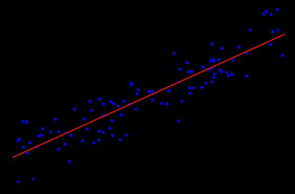
It looks very similar to a system of linear equations, doesn't it? It seems so, but solutions to such a system of equations are likely to not exist. The reason for this is the noise that is present in almost any real data. Additionally, a lack of linear dependence as such may exist, which can be attempted to be mitigated by introducing additional variables that are non-linearly related to the originals. Consider the following example:
Source:
This is a simple example of linear regression that demonstrates the dependence of one variable (on the axis  ) on another variable (on the axis
  ). For the corresponding system of linear equations to have a solution, all points must lie exactly on one line. However, this is not the case. They do not lie on one line precisely because of noise (or due to the erroneous assumption of a linear dependence). Thus, to restore linear dependence from real data, it is usually necessary to introduce another assumption: the input data contains noise and this noise has . Assumptions can also be made about other types of noise distributions, but in the overwhelming majority of cases, normal distribution is considered, which will be discussed further.
Maximum Likelihood Method
. So, we have assumed the presence of randomly normally distributed noise. What should we do in such a situation? In mathematics, there is a method that is widely used for this . In short, its essence lies in choosing and subsequently maximizing it.
Returning to the restoration of linear dependence from data with normal noise. Note that the assumed linear dependence is the mathematical expectation of  the existing normal distribution. At the same time, the probability that
  takes on certain values, given the presence of observed
  , looks as follows:

Now, let's substitute in place of  and
and  the variables we need:

We just need to find the vector  , at which this probability is maximized. To maximize such a function, it is convenient to logarithmically transform it first (the logarithm of the function will reach its maximum at the same point as the function itself):

This, in turn, reduces to minimizing the following function:

By the way, this is called the . Often, all the above reasoning is omitted, and this method is simply used.
QR decomposition
The minimum of the function presented above can be found by locating the point at which the gradient of this function is zero. The gradient will be expressed as follows:

is a matrix method for solving minimization problems used in the least squares method. In this regard, let’s rewrite the equation in matrix form:

So, we decompose the matrix  into matrices
  and
and  and performing a number of transformations (the QR decomposition algorithm itself will not be discussed here, only its application to the given task):

Matrix  is orthogonal. This allows us to eliminate the product of
  :
:

And if we replace  to
to  , it will result in
  . Considering that
  is an upper triangular matrix, this looks as follows:

This can be solved using the substitution method. The element  is determined as
  , the previous element
  is determined as
  and so on.
It is worth noting that the complexity of the resulting algorithm due to the use of QR decomposition is equal to  . However, despite the fact that the matrix multiplication operation is well-parallelized, writing an efficient distributed version of this algorithm is not feasible.
Gradient descent
When discussing the minimization of a certain function, it's always important to recall the method of (stochastic) gradient descent. It is a simple and effective minimization method based on iteratively calculating the gradient of the function at a point and subsequently shifting it in the opposite direction of the gradient. Each such step brings the solution closer to the minimum. The gradient at this point looks like this:

Moreover, this method is well-parallelized and distributed due to the linear properties of the gradient operator. Note that in the formula above, the terms under the summation sign are independent. In other words, we can calculate the gradient independently for all indices  from the first to
  , while simultaneously calculating the gradient for indices from
  up to
up to  . We then sum the resulting gradients together. The sum will be the same as if we calculated the gradient directly for the indices from the first to
  . Thus, if the data is distributed among several data partitions, the gradient can be computed independently on each partition, and then the results of these computations can be summed to obtain the final result:

From an implementation perspective, this fits into the paradigm of . At each step of the gradient descent, a task is sent to each data node to compute the gradient, then the computed gradients are collected together, and the result of their summation is used to improve the outcome.
Despite its simplicity of implementation and the ability to operate in the MapReduce paradigm, gradient descent has its drawbacks. In particular, the number of steps required to achieve convergence is significantly higher compared to other more specialized methods.
LSQR
is another method for solving the given problem, suitable for both linear regression recovery and solving systems of linear equations. Its main feature is that it combines the advantages of matrix methods and an iterative approach. Implementations of this method can be found in libraries like , and in . A description of this method will not be provided here (it can be found in the article ). Instead, an approach will be demonstrated that allows adapting LSQR for execution in a distributed environment.
The LSQR method is based on the . This is an iterative procedure, where each iteration consists of the following steps:
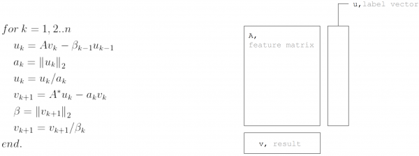
However, assuming that the matrix is  horizontally partitioned, each iteration can be represented as two MapReduce steps. This allows minimizing data transfer during each iteration (only vectors of length equal to the number of unknowns):
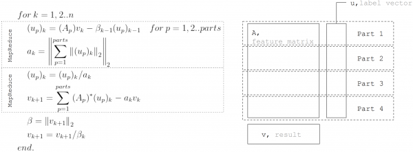
This approach is used when implementing linear regression in .
Conclusion
There are many algorithms for recovering linear regression, but not all of them can be applied under any conditions. For example, QR decomposition is excellent for exact solutions on small datasets. Gradient descent is straightforward to implement and allows for quickly finding approximate solutions. LSQR combines the best properties of the previous two algorithms as it can be distributed, converges faster than gradient descent, and also allows for an early stopping of the algorithm compared to QR decomposition for finding approximate solutions.
Source: habr.com
