🥇Chewing over logistic regression

In this article, we will analyze the theoretical foundations of transformation. the linear regression function. downward API support (simultaneously with this in the inverse logit transformation function (also referred to as the logistic response function).Then, using the arsenal of the maximum likelihood method,according to the logistic regression model, we will derive the loss function. Logistic Loss,or in other words, we will determine the function through which the parameters of the weight vector are fitted in the logistic regression model. .

Article Outline:

Let's revisit the linear relationship between two variables.
We will identify the need for transformation of the linear regression function. downward API support (simultaneously with this in the logistic response function.
We will perform transformations and derive the logistic response function.
We will try to understand why the least squares method is inadequate for parameter fitting functions Logistic Loss,
We use maximum likelihood method to determine the parameter fitting function. :
5.1. Case 1: function Logistic Loss, for objects with class labels. 0 and 1:

5.2. Case 2: function Logistic Loss, for objects with class labels. -1 and +1:

The article is filled with simple examples where all calculations can be easily performed mentally or on paper; in some cases, a calculator may be needed. So be prepared 🙂

This article is primarily aimed at data scientists with a basic understanding of machine learning fundamentals.

The article will also provide code for plotting graphs and calculations. All code is written in the python 2.7language. I will clarify in advance the 'novelty' of the version used—this is one of the conditions for passing a well-known course from Yandex, on a well-known online education platform, Courseraand, as can be assumed, the material was prepared based on this course.

01. Linear dependence

It is quite reasonable to ask the question—what is the connection between linear dependence and logistic regression?

It's simple! Logistic regression is one of the models that fall under the linear classifier category. In simple terms, the task of a linear classifier is to predict target values from variables (regressors). It is assumed that the relationship between the features and the target values is linear. Hence the name of the classifier—it is linear. If we generalize significantly, the basis of the logistic regression model rests on the assumption of a linear relationship between the features. and the target values is Here it is—the connection.

In the studio, the first example is indeed about the linear dependency of the studied quantities. While preparing the article, I stumbled upon an example that has become rather clichéd — the dependency of current on voltage. (“Applied Regression Analysis,” N. Draper, G. Smith). Here, we will also consider it.

In accordance with Ohm's law:

, where — current, — voltage, — resistance.

If we didn’t know Ohm's law, we could find the dependency empirically, changing and measuring , keeping fixed. Then we would see that the graph of the dependency from gives a more or less straight line passing through the origin. We said 'more or less,' since although the dependency is actually exact, our measurements may contain small errors, and thus the points on the graph may not fall strictly on the line but be scattered around it randomly.

Graph 1: ‘Dependency from »

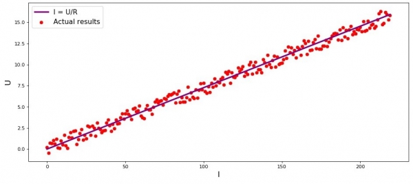
Graph Rendering Code

import matplotlib.pyplot as plt
%matplotlib inline

import numpy as np

import random

R = 13.75

x_line = np.arange(0,220,1)
y_line = []
for i in x_line:
    y_line.append(i/R)
    
y_dot = []
for i in y_line:
    y_dot.append(i+random.uniform(-0.9,0.9))


fig, axes = plt.subplots(figsize = (14,6), dpi = 80)
plt.plot(x_line,y_line,color = 'purple',lw = 3, label = 'I = U/R')
plt.scatter(x_line,y_dot,color = 'red', label = 'Actual results')
plt.xlabel('I', size = 16)
plt.ylabel('U', size = 16)
plt.legend(prop = {'size': 14})
plt.show()

02. The Necessity of Transformations of the Linear Regression Equation

Let’s consider another example. Imagine that we work in a bank, and our task is to determine the probability of a borrower repaying a loan based on certain factors. To simplify the task, we will consider just two factors: the borrower’s monthly salary and the monthly payment amount for loan repayment.

The task is very conditional, but with this example, we will understand why applying the linear regression function., and we will also learn what transformations need to be made to the function.

Returning to the example. It is understood that the higher the salary, the more the borrower can allocate monthly for loan repayment. At the same time, for a certain salary range, this relationship will be quite linear. For instance, let’s take a salary range from 60,000 RUB to 200,000 RUB and assume that within this salary range, the relationship between the size of the monthly payment and the size of the salary is linear. Let’s suppose that it has been determined for this salary range that the ratio of salary to payment should not fall below 3, and the borrower should also have 5,000 RUB in reserve. Only in this case will we consider that the borrower will repay the loan to the bank. Then, the linear regression equation will look like this:

where , , , — the borrower's salary, the loan payment — of the borrower. Substituting the salary and loan payment into the equation with fixed parameters

a decision can be made to approve or refuse the loan. Looking ahead, we note that, with the given parameters,

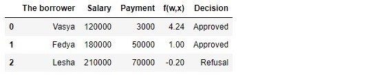
the linear regression function , used inthe logistic response function will yield high values, which complicate calculations for determining the probabilities of loan repayment. Therefore, it is suggested to reduce our coefficients, let’s say, by 25,000 times. This transformation in coefficients will not change the decision regarding the loan issuance. Let’s remember this point for the future, and now, to clarify what we are talking about, let’s consider the situation with three potential borrowers. Table 1 "Potential Borrowers"

Code to generate the table

import pandas as pdr = 25000.0 w_0 = -5000.0/r w_1 = 1.0/r w_2 = -3.0/rdata = {'The borrower':np.array(['Vasya', 'Fedya', 'Lesha']), 'Salary':np.array([120000,180000,210000]), 'Payment':np.array([3000,50000,70000])}df = pd.DataFrame(data)df['f(w,x)'] = w_0 + df['Salary']*w_1 + df['Payment']*w_2decision = [] for i in df['f(w,x)']: if i > 0: dec = 'Approved' decision.append(dec) else: dec = 'Refusal' decision.append(dec) df['Decision'] = decisiondf[['The borrower', 'Salary', 'Payment', 'f(w,x)', 'Decision']]

According to the data in the table, Vasya, with a salary of 120,000 RUB, wants to take a loan that he will repay at 3,000 RUB monthly. We have determined that for the loan to be approved, Vasya's salary must be three times greater than the payment, and he should still have 5,000 RUB left. This requirement is satisfied by Vasya:

According to the data in the table, Vasya, with a salary of 120,000 RUB, wants to obtain a loan such that his monthly repayment is 3,000 RUB. We have determined that to approve the loan, Vasya's salary must exceed three times the payment amount and still leave him with 5,000 RUB. Vasya meets this requirement: There remains even 106,000 R. Despite the fact that we reduced the coefficients by 25,000 times, we obtained the same result — the loan can be approved. Fedya will also receive a loan, while Lesha, despite earning the most, will have to moderate his appetites. 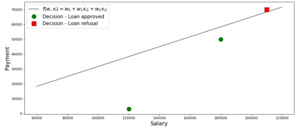Let's draw a graph on this occasion.

Graph 2 "Classification of Borrowers"

Code to draw the graph

salary = np.arange(60000,240000,20000) payment = (-w_0-w_1*salary)/w_2fig, axes = plt.subplots(figsize=(14,6), dpi=80) plt.plot(salary, payment, color='grey', lw=2, label='$f(w,x_i)=w_0 + w_1x_{i1} + w_2x_{i2}$') plt.plot(df[df['Decision'] == 'Approved']['Salary'], df[df['Decision'] == 'Approved']['Payment'], 'o', color='green', markersize=12, label='Decision - Loan approved') plt.plot(df[df['Decision'] == 'Refusal']['Salary'], df[df['Decision'] == 'Refusal']['Payment'], 's', color='red', markersize=12, label='Decision - Loan refusal') plt.xlabel('Salary', size=16) plt.ylabel('Payment', size=16) plt.legend(prop={'size': 14}) plt.show()

So, our line, built according to the function

, separates "bad" borrowers from "good" ones. Borrowers whose desires do not match their capabilities are above the line (Lesha), while those capable of repaying the loan according to our model parameters are below the line (Vasya and Fedya). In other words, our line divides borrowers into two classes. We will denote them as follows: we will assign to the class those borrowers who are most likely to repay the loan, and to the class those borrowers who are most likely unable to repay the loan. or Let's generalize the conclusions from this simple example. Let's take a point

and, by substituting the coordinates of the point into the corresponding equation of the line , consider three options: If the point is below the line, and we classify it as belonging to class

, then the value of the function will be positive from . Thus, we can consider that the probability of loan repayment is within up to . The higher the value of the function, the greater the probability. If the point is above the line and we classify it as belonging to class
, the value of the function will be negative from or . Then we will consider that the probability of repayment is within up to and the greater the absolute value of the function, the higher our confidence. The point lies on the line, on the boundary between the two classes. In this case, the value of the function
will be equal to and the probability of loan repayment is Now, imagine that we have not two factors, but dozens, and instead of three borrowers, we have thousands. Then instead of a line, we will have .

Now, let’s imagine that we have not two factors, but dozens, and instead of three borrowers, we have thousands. Then instead of a line, we will have Logit plane and coefficients we will use values derived from well-established rules based on accumulated data about borrowers, whether they repaid or defaulted on their loans. Indeed, notice that we are currently selecting borrowers using already known coefficients . The task of the logistic regression model is precisely to determine the parameters , at which the loss function value Logistic Loss, will tend to a minimum. But how the vector is calculated , we will learn in Section 5 of the article. For now, let's return to the Promised Land — to our banker and his three clients.

Thanks to the function we know who can be granted a loan and who should be denied. But we cannot approach the director with such information, because they wanted us to provide the probability of each borrower repaying the loan. What to do? The answer is simple — we need to somehow transform the function , with values lying in the range to a function that will have values in the range . Such a function exists; it is called the logistic response function or the inverse logit transformation. Meet:

Let's look at the steps of how the logistic response functionis obtained. Note that we will proceed in reverse, i.e., we will assume that we know the probability value, which lies within the limits of up to , and then we will 'unwind' this value across the entire number range from up to .

03. We derive the logistic response function.

Step 1. We will translate the probability values into the range

During the function transformation, downward API support (simultaneously with this in the logistic response function. we will leave our credit analyst alone and instead take a look at the bookmakers. No, of course, we won't be placing bets; all we are interested in is the meaning of the expression, for example, a chance of 4 to 1. The odds, familiar to all bettors, represent a ratio of 'successes' to 'failures.' From a probability perspective, odds are the probability of an event occurring divided by the probability that the event does not occur. Let's write the formula for the odds of an event occurring: :

, where — the probability of the event occurring, — the probability of the event NOT occurring

For example, if the probability of a young, strong, and agile horse nicknamed 'Wind' outpacing an old, flabby mare named 'Matilda' is , the odds of 'Wind' succeeding will be to , and conversely, knowing the odds allows us to easily calculate the probability :

. Thus, we have learned to 'translate' probability into odds, which can take values from up to . Let's take another step and learn to 'translate' probability across the entire number line from up to .

Step 2. We will translate probability values into the range

This step is very simple — we will logarithmically transform the odds with base Euler's number and obtain:

Now we know that if , calculating the value of will be very straightforward and, moreover, it should be positive: . Indeed, it is.

Out of curiosity, let's check what happens if , then we expect to see a negative value . Let's verify: . That's correct.

Now we know how to translate the probability value from up to across the entire number line from up to . In the next step, we will do everything in reverse.

For now, let's note that according to the rules of logarithmization, knowing the value of the function , we can calculate the odds:

This method of determining odds will be useful in the next step.

Step 3. Let's derive the formula for determining

So, we have learned to find the values of the function , knowing that . However, what we actually need is precisely the opposite — knowing the value of to find . For this, we will turn to the concept of the inverse odds function, according to which:

In this article, we will not derive the aforementioned formula, but will check with the numbers from the earlier example. We know that with odds of 4 to 1 (), the probability of the event occurring is 0.8 (). Let's substitute: . This matches our calculations performed earlier. Let's move forward.

In the previous step, we derived that , so we can make a substitution in the inverse odds function. We get:

Dividing both the numerator and denominator by , then:

Just in case, to ensure we haven't made any mistakes, let's perform one more small check. In Step 2, we determined that . Then, substituting the value into the logistic response function, we expect to get . Substituting it in, we get: .

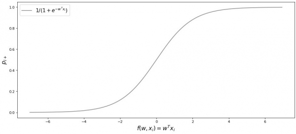
Congratulations, dear reader, we have just derived and tested the logistic function. Let's take a look at the function graph.

Figure 3 "Logistic Function"

import math

def logit(f):
    return 1/(1+math.exp(-f))

f = np.arange(-7,7,0.05)
p = []

for i in f:
    p.append(logit(i))

fig, axes = plt.subplots(figsize=(14,6), dpi=80)
plt.plot(f, p, color='grey', label='$ 1 / (1+e^{-w^Tx_i})$')
plt.xlabel('$f(w,x_i) = w^Tx_i$', size=16)
plt.ylabel('$p_{i+}$', size=16)
plt.legend(prop={'size': 14})
plt.show()

In the literature, this function can also be referred to as the sigmoid function. The graph clearly shows that the main change in the probability of an object belonging to a class occurs within a relatively small range , somewhere from up to .

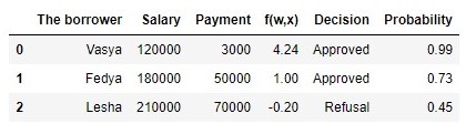
I suggest we return to our credit analyst and help him calculate the probability of loan repayments, otherwise he risks not receiving his bonus 🙂

Table 2 "Potential Borrowers"

proba = []
for i in df['f(w,x)']:
    proba.append(round(logit(i), 2))
    
df['Probability'] = proba

df[['The borrower', 'Salary', 'Payment', 'f(w,x)', 'Decision', 'Probability']]

So, we have determined the probability of loan repayment. Overall, it seems to hold true.

Indeed, the probability that Vasya will be able to pay the bank 3,000 R per month with a salary of 120,000 R is close to 100%. By the way, we need to understand that the bank can also issue a loan to Lesha if the bank's policies allow, for example, lending to clients with a probability of loan repayment greater than, let's say, 0.3. In such a case, the bank would simply create a larger reserve for potential losses.

It should also be noted that the ratio of salary to payment being no less than 3, and with a buffer of 5,000 R was somewhat arbitrary. Therefore, we couldn’t use the weight vector in its original form. We needed to significantly reduce the coefficients, and in this scenario, we divided each coefficient by 25,000, essentially adjusting the result. This was done specifically to simplify the understanding of the material at the initial stage. In real life, we will need to find the coefficients, not concoct and adjust them. In the following sections of the article, we will derive equations that help in selecting parameters. .

04. The Method of Least Squares for Determining the Weight Vector in the logistic function

We are already familiar with such a method for selecting the weight vector as a the method of least squares (OLS) So, why shouldn’t we use it in binary classification tasks? Indeed, nothing prevents us from using it. LSMHowever, this method yields less accurate results in classification tasks than. Logistic Loss,There is a theoretical justification for this. Let’s start by looking at a simple example.

Let’s assume our models (using MSE and Logistic Loss,) have already begun weight vector selection. And we stopped the calculation at some step. It doesn’t matter whether it’s in the middle, at the end, or at the beginning; what’s important is that we already have some weight vector values. Let’s suppose that at this step, the weight vectors for both models are identical. In that case, let’s take the obtained weights and substitute them into the logistic response function. () for some object that belongs to the class . We will explore two scenarios: when, based on the selected weight vector, our model makes significant errors, and conversely, when the model is very confident that the object belongs to class . Let’s see what penalties are assigned when using LSM and Logistic Loss,.

Code for calculating penalties based on the chosen loss function.

# класс объекта
y = 1
# вероятность отнесения объекта к классу в соответствии с параметрами w
proba_1 = 0.01

MSE_1 = (y - proba_1)**2
print 'Штраф MSE при грубой ошибке =', MSE_1

# напишем функцию для вычисления f(w,x) при известной вероятности отнесения объекта к классу +1 (f(w,x)=ln(odds+))
def f_w_x(proba):
    return math.log(proba/(1-proba)) 

LogLoss_1 = math.log(1+math.exp(-y*f_w_x(proba_1)))
print 'Штраф Log Loss при грубой ошибке =', LogLoss_1

proba_2 = 0.99

MSE_2 = (y - proba_2)**2
LogLoss_2 = math.log(1+math.exp(-y*f_w_x(proba_2)))

print '**************************************************************'
print 'Штраф MSE при сильной уверенности =', MSE_2
print 'Штраф Log Loss при сильной уверенности =', LogLoss_2

The case of a gross error — the model classifies the object as belonging to class with a probability of 0.01.

The penalty when using LSM will be:

The penalty when using Logistic Loss, will be:

The case of strong confidence — the model classifies the object as belonging to class with a probability of 0.99.

The penalty when using LSM will be:

The penalty when using Logistic Loss, will be:

This example illustrates well that in the case of a gross error, the loss function Log Loss penalizes the model much more heavily than. MSENow let’s understand the theoretical prerequisites for using the loss function Log Loss in classification tasks.

05. Maximum Likelihood Method and Logistic Regression

As promised at the beginning, the article abounds with simple examples. Here’s another example with our old guests — bank borrowers: Vasya, Fedia, and Lesha.

Just in case, before developing the example, let me remind you that in real life we deal with a training dataset of thousands or millions of objects with dozens or hundreds of features. However, the numbers here are chosen to be easily manageable for a novice data scientist.

Let's return to the example. Imagine that the bank director decided to grant loans to everyone in need, despite the algorithm suggesting not to issue one to Alex. Time has passed, and we know who among the three heroes repaid the loan and who did not. As expected, Vasya and Fedya repaid the loan, while Alex did not. Now, let’s consider that this outcome will serve as our new training sample, while all data regarding the factors influencing loan repayment probability (borrower's salary, size of the monthly payment) have seemingly disappeared. Intuitively, we might assume that every third borrower does not return the loan or, in other words, the probability of the next borrower repaying the loan. This intuitive assumption has theoretical confirmation and is based on the method of maximum likelihood, often referred to in literature as the principle of maximum likelihood..

First, let's get acquainted with the conceptual apparatus.

The likelihood of the sample is the probability of obtaining exactly this sample, obtaining exactly such observations/results, i.e., the product of the probabilities of obtaining each of the results of the sample (for example, whether the loan was repaid or not by Vasya, Fedya, and Alex simultaneously).

The likelihood function links the sample likelihood with the values of the distribution parameters.

In our case, the training sample represents a generalized Bernoulli scheme, in which the random variable takes only two values: or . Therefore, the likelihood of the sample can be expressed as a likelihood function of the parameter as follows:

The above expression can be interpreted as follows. The joint probability that Vasya and Fedya will repay the loan is equal to , the probability that Alex did NOT repay the loan is equal to (since it was specifically the case of NOT repaying the loan), thus the joint probability of all three events is equal to .

Maximum Likelihood Method — this is a method for estimating an unknown parameter by maximizing the likelihood function. In our case, it is necessary to find such a value , at which achieves its maximum.

Where does the idea of searching for the value of an unknown parameter, at which the likelihood function reaches its maximum, come from? The origins of this idea stem from the understanding that a sample is the only source of knowledge we have about the population. Everything we know about the population is represented in the sample. Therefore, all we can say is that the sample is the most accurate reflection of the population available to us. Consequently, we need to find such a parameter at which the given sample becomes the most probable.

It is evident that we are dealing with an optimization problem in which we need to find the extremum point of the function. To find this extremum point, it is necessary to consider the first-order condition, that is, to equate the derivative of the function to zero and solve the equation for the unknown parameter. However, searching for the derivative of a product involving many factors can be a lengthy process; to avoid this, there is a special technique — transitioning to the logarithm. the likelihood function. Why is such a transition possible? Let's note that we are not looking for the extremum of the function itself,, but rather the extremum point, that is, the value of the unknown parameter , at which that reaches its maximum. When transitioning to the logarithm, the extremum point does not change (although the extremum itself will differ) since the logarithm is a monotonic function.

Let us continue to develop our example with loans from Vasya, Fedya, and Lesha, following the above. Let's transition to the logarithm of the likelihood function.:

Now we can easily differentiate the expression with respect to :

And finally, let us consider the first-order condition — we set the derivative of the function to zero:

Thus, our intuitive estimate of the probability of loan repayment has been theoretically justified.

Great, but what do we do with this information now? If we assume that every third borrower will not repay the bank, it will inevitably go bankrupt. It sounds reasonable, but when estimating the probability of loan repayment as equal to We did not consider the factors affecting the loan repayment: the borrower's salary and the size of the monthly payment. Recall that earlier we calculated the probability of loan repayment for each client, taking these very factors into account. It is logical that our probabilities turned out to be different from the constant value of .

Let's define the likelihood of the samples:

Code for calculating the likelihood of the samples

from functools import reduce

def likelihood(y,p):
    line_true_proba = []
    for i in range(len(y)):
        ltp_i = p[i]**y[i]*(1-p[i])**(1-y[i])
        line_true_proba.append(ltp_i)
    likelihood = []
    return reduce(lambda a, b: a*b, line_true_proba)
        
    
y = [1.0,1.0,0.0]
p_log_response = df['Probability']
const = 2.0/3.0
p_const = [const, const, const]


print 'Sample likelihood at constant p=2/3:', round(likelihood(y,p_const),3)

print '****************************************************************************************************'

print 'Sample likelihood at calculated p value:', round(likelihood(y,p_log_response),3)

The likelihood of the sample at a constant value :

The likelihood of the sample when calculating the loan repayment probability considering the factors :

The likelihood of the sample, with the probability calculated based on the factors, turned out to be higher than the likelihood at the constant probability value. What does this mean? It means that knowledge of the factors allowed for a more accurate selection of the loan repayment probability for each client. Therefore, when issuing another loan, it would be more appropriate to use the model for estimating repayment probability proposed at the end of Section 3 of the article.

But then, if we need to maximize the likelihood function of the sample, why not use some algorithm that would provide probabilities for Vasya, Fedya, and Lesha, for example, equal to 0.99, 0.99, and 0.01, respectively? Such an algorithm might perform well on the training sample, as it would bring the value of the sample likelihood closer to , but, firstly, such an algorithm is likely to have difficulties with generalization ability; secondly, this algorithm will definitely not be linear. And if methods for combating overfitting (as well as weak generalization ability) are clearly not part of this article's plan, then let’s delve into the second point in more detail. To do this, it's enough to answer a simple question. Can the probability of loan repayment for Vasya and Fedya be the same, considering the factors we know? From a commonsense perspective, of course not, it cannot. Thus, Vasya will be paying 2.5% of his salary monthly towards the loan, while Fedya will be paying almost 27.8%. Also, in Figure 2 'Customer Classification,' we see that Vasya is significantly further from the decision boundary than Fedya. Finally, we know that the function for Vasya and Fedya takes different values: 4.24 for Vasya and 1.0 for Fedya. If, for example, Fedya earned an order of magnitude more or asked for a smaller loan, then the probabilities of loan repayment for Vasya and Fedya would be similar. In other words, you can't deceive a linear dependence. And if we had indeed calculated the coefficients , rather than pulled them out of thin air, we could confidently say that our values are best suited to estimate the probability of loan repayment by each borrower; however, since we have agreed to assume that the determination of the coefficients was carried out according to all the rules, we will maintain that our coefficients provide the best estimate of the probability 🙂

However, we got sidetracked. In this section, we need to figure out how the weight vector is determined , which is necessary for assessing the probability of loan return by each borrower.

In short, let's summarize what arsenal we are bringing to the search for coefficients :

1. We assume that the relationship between the target variable (predicted value) and the factor influencing the result is linear. For this reason, a model of the type , used in is applied, the line of which divides the objects (clients) into classes (clients capable of repaying the loan and those who are not). In our case, the equation looks like and or 2. We use .

the inverse logit transformation function to determine the probability of an object belonging to a class is applied, the line of which divides the objects (clients) into classes 3. We consider our training sample as a realization of the generalized .

3. We consider our training sample as the realization of a generalized Bernoulli schemes, meaning that for each object a random variable is generated, which with a probability of (its own for each object) takes the value of 1 and with a probability of – 0.

4. We know that we need to maximize the likelihood function of the sample given the accepted factors so that the existing sample becomes the most plausible. In other words, we need to find parameters such that the sample will be the most plausible. In our case, the parameter being optimized is the probability of loan repayment , which in turn depends on unknown coefficients . Therefore, we need to find such a weight vector , for which the likelihood of the sample will be maximized.

5. We know that to maximize the likelihood function of the sample you can use maximum likelihood method. And we know all the clever tricks for working with this method.

This is quite a complex situation 🙂

Now let’s remember that at the very beginning of the article we wanted to derive two types of loss functions Logistic Loss, depending on how the object classes are designated. It is customary in classification tasks with two classes to denote the classes as and or . Depending on the designation, the corresponding loss function will be produced.

Case 1. Classification of objects into and

Previously, when determining the sample's likelihood, where the probability of default by the borrower was calculated based on factors and given coefficients , we applied the formula:

In fact, — this is the value of the logistic response function given a specified weight vector

Then nothing prevents us from writing the likelihood function of the sample as follows:

Sometimes it happens that some novice analysts find it difficult to immediately understand how this function works. Let's consider 4 brief examples that will clarify everything:

1. If (i.e., according to the training sample, the object belongs to class +1), while our algorithm determines the probability of the object belonging to the class as 0.9, then this piece of the sample's likelihood will be calculated as follows:

2. If , and , then the calculation will be as follows:

3. If , and , then the calculation will be as follows:

4. If , and , then the calculation will be as follows:

It is obvious that the likelihood function will be maximized in cases 1 and 3, or in general — when the probabilities of an object belonging to the class are correctly guessed. .

Due to the fact that when determining the probability of assigning an object to a class We only do not know the coefficients , so we will look for them. As mentioned above, this is an optimization task, where initially we need to find the derivative of the likelihood function with respect to the weight vector . However, it makes sense to simplify the task beforehand: we will seek the derivative of the logarithm the likelihood function.

Why after logarithmization, in the logistic loss function, we changed the sign from to . It's simple, because in tasks involving model quality assessment it is customary to minimize the value of the function, so we multiplied the right side of the expression by and accordingly, instead of maximizing, we now minimize the function.

Actually, right now, in front of your eyes, a loss function has been painfully derived — Logistic Loss, for the training sample with two classes: and .

Now, to find the coefficients, we just need to find the derivative the logistic loss function and then, using numerical optimization methods like gradient descent or stochastic gradient descent, find the most optimal coefficients . But, considering the already significant volume of the article, it is suggested to perform differentiation independently or, perhaps, this will be the topic for the next article with a lot of arithmetic without such detailed examples.

Case 2. Classification of objects in and

The approach here will be the same as with classes and , but the path to deriving the loss function Logistic Loss,, will be more convoluted. Let's get started. We will use the operator for the likelihood function "if..., then...". That is, if the object belongs to class , then for calculating the likelihood of the sample we use the probability , if the object belongs to class , then we substitute into the likelihood. This is what the likelihood function looks like:

In simple terms, let's outline how this works. Consider 4 cases:

1. If and , then in the likelihood of the sample it will be

2. If and , then in the likelihood of the sample it will be

3. If and , then in the likelihood of the sample it will be

4. If and , then in the likelihood of the sample it will be

It is obvious that in cases 1 and 3, when the probabilities were correctly defined by the algorithm, the likelihood function will be maximized, which is exactly what we wanted to achieve. However, this approach is quite cumbersome, and we will consider a more compact notation afterwards. But first, let's logarithmically transform the likelihood function by changing the sign since we will minimize it now.

Instead of substituting the expression :

Let's simplify the right summand under the logarithm using basic arithmetic techniques and get:

Now it's time to get rid of the operator "if..., then...". Note that when an object belongs to the class , in the expression under the logarithm, in the denominator, is raised to the power , if the object belongs to class , then $e$ is raised to the power . Therefore, the power expression can be simplified — we can combine both cases into one: . Thus, the logistic loss function will take the form: