

"If you read 'buffalo' on the elephant's cage, don't trust your eyes" - Kozma Prutkov
In the previous it was shown why an object model is necessary and proved that without this object model, one can only speak of model-based design as a marketing gimmick, meaningless and merciless. However, once the object model is presented, competent engineers always raise a reasonable question: what evidence is there that the mathematical model of the object corresponds to the real object.

One example of an answer to this question is presented in In this article, we will examine an example of creating a model for aviation air conditioning systems, mixing practice with some theoretical considerations of a general nature.
Creating a reliable object model. Theory
To get straight to the point, I will immediately outline the algorithm for creating a model for model-oriented design. It consists of just three simple steps:
Step 1. Develop a system of algebraic-differential equations describing the dynamic behavior of the modeled system. This is straightforward if you know the physics of the process. Many researchers have already developed for us the basic physical laws by Newton, Bernoulli, Navier-Stokes, and others.
Step 2. Identify in the resulting system a set of empirical coefficients and characteristics of the modeling object that can be obtained from tests.
Step 3. Conduct tests on the object and adjust the model based on the results of real experiments so that it corresponds to reality, with the necessary degree of detail.
As you can see, it's as simple as one, two, three.
An example of practical implementation
The air conditioning system (ACS) in an aircraft is connected to the automatic pressure maintenance system. The pressure in the aircraft must always be greater than the external pressure, and the rate of pressure change should be such that neither the pilots nor the passengers experience nosebleeds or ear issues. Therefore, the control system for air intake and outflow is crucial for safety, and its development on the ground involves expensive testing systems. These systems create flight altitude temperatures and pressures, simulating takeoff and landing modes at airfields of varying heights. The challenge of developing and fine-tuning the control systems for the ACS comes to the forefront. How long will we run the test stand to achieve a satisfactory control system? Clearly, if we tune the control model on the object model, the work cycle on the test stand can be significantly reduced.
The aviation air conditioning system consists of heat exchangers similar to those in any other thermal system. A battery is a battery, even in Africa, just a different kind of air conditioner. However, due to constraints on takeoff weight and dimensions of aircraft, heat exchangers are made as compact and efficient as possible to transfer as much heat as possible with minimal weight. As a result, the geometry can become quite intricate. For instance, in the case under consideration, Figure 1 shows a plate heat exchanger that employs a membrane between the plates to enhance heat exchange. Hot and cold heat carriers alternate in the channels, with the flow direction being transverse. One heat carrier is supplied to the front edge, while the other is supplied to the side.
To solve the control problem of the ACS, we need to determine how much heat is transferred from one medium to another through such a heat exchanger per unit time. This affects the rate of temperature change, which we are regulating.
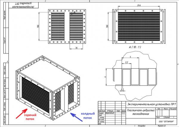
Figure 1. Schematic of an aviation heat exchanger.
Modeling Issues. Hydraulic Component
At first glance, the task seems quite simple: it is necessary to calculate the mass flow through the channels of the heat exchanger and the thermal flow between the channels.
The mass flow rate of the heat carrier in the channels is calculated using Bernoulli's formula:
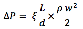
where:
ΔP – the pressure drop between two points;
ξ – the friction coefficient of the heat carrier;
L – the length of the channel;
d – the hydraulic diameter of the channel;
ρ – the density of the heat carrier;
ω – the velocity of the heat carrier in the channel.
For a channel of arbitrary shape, the hydraulic diameter is calculated using the formula:

where:
F – the cross-sectional area;
P – the wetted perimeter of the channel.
The friction coefficient is calculated using empirical formulas and depends on the flow velocity and properties of the heat carrier. Different geometries result in different dependencies; for example, the formula for turbulent flow in smooth pipes is:
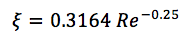
where:
Re – Reynolds number.
For flow in flat channels, the following formula can be used:

From Bernoulli's formula, one can calculate the pressure drop for a given velocity, or conversely, to calculate the velocity of the heat carrier in the channel based on a given pressure drop.
Heat Exchange
The heat flux between the heat carrier and the wall is calculated using the formula:

where:
α [W/(m²×°C)] – the heat transfer coefficient;
F – the cross-sectional area.
For the problems of flow of heat carriers in pipes, a sufficient number of studies have been conducted, and there are many calculation methods available, which usually boil down to empirical dependencies for the heat transfer coefficient α [W/(m²×°C)]
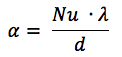
where:
Nu – Nusselt number,
λ – thermal conductivity coefficient of the liquid [W/(m×°C)]
d – the hydraulic (equivalent) diameter.
To calculate the Nusselt number (criteria), empirical correlational dependencies are used; for example, the formula for calculating the Nusselt number in a round pipe is as follows:

Here we already see the Reynolds number, the Prandtl number at the wall temperature and the liquid temperature, and the non-uniformity coefficient. ()
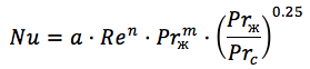
For plate heat exchangers, the formula is similar ( ):
where:
n = 0.73 m = 0.43 for turbulent flow,
coefficient a – varies between 0.065 and 0.6 depending on the number of plates and flow regime.
Let's note that this coefficient is calculated only for one point in the flow. For the next point, we have a different liquid temperature (it has either heated up or cooled down), a different wall temperature, and, accordingly, all the Reynolds numbers and Prandtl numbers change.
At this point, any mathematician will say that it is impossible to calculate the system accurately when the coefficient changes by a factor of 10, and they would be right.
Any practical engineer will say that each heat exchanger varies during manufacturing and that calculating systems is impossible, and they would also be right.
But what about model-based design? Is everything lost?
Savvy vendors of Western software will try to sell you Supercomputers and 3D calculation systems here, claiming that it's impossible without them. And you need to run calculations for a day to get the temperature distribution over just 1 minute.
It's clear that this isn't our option; we need to debug the control system, if not in real time, then at least within a reasonable timeframe.
A trial-and-error solution.
A heat exchanger is manufactured, a series of tests are conducted, and a table of efficiency is established for the steady-state temperature at given heat transfer rates. Simple, fast, and reliable, as the data is obtained from experiments.
The downside of this approach is that there are no dynamic characteristics of the object. Yes, we know what the steady-state heat flux will be, but we do not know how long it will take to reach that state when transitioning from one operating mode to another.
Therefore, after calculating the necessary characteristics, we tune the control system directly during the tests, which is what we initially wanted to avoid.
Model-oriented approach.
To create a model of a dynamic heat exchanger, it is necessary to use data from tests to eliminate uncertainties in the empirical calculation formulas - Nusselt numbers and hydraulic resistance.
The solution is as simple as all genius ideas. We take the empirical formula, conduct experiments, and determine the value of coefficient a, thereby eliminating the uncertainty in the formula.
Once we have a certain value of the heat transfer coefficient, all other parameters are determined by the basic physical laws of conservation. The temperature difference and the heat transfer coefficient define the amount of energy transferred to the channel per unit time.
Knowing the energy flow, we can solve the energy, mass conservation, and momentum equations for the heat transfer fluid in a hydraulic channel. For example, such as:

In our case, the heat flow between the wall and the heat carrier remains undefined — Qwall. More details can be found
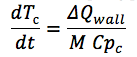
And also the temperature derivative equation for the channel wall:
where:
ΔQwall – the difference between the incoming and outgoing flow at the channel wall;
M – the mass of the channel wall;
Cpc – the heat capacity of the wall material.
Model Accuracy
As mentioned above, in the heat exchanger we have a temperature distribution across the surface of the plate. For steady-state values, one can take the average across the plates and use it, representing the entire heat exchanger as a single concentrated point where, at one temperature difference, heat is transferred across the entire surface of the heat exchanger. However, for transient modes, such an approximation may not work. The other extreme is to create several hundred thousand points and overload a supercomputer, which also does not suit us, as the task is to tune the control system in real-time, preferably faster.
The question arises, into how many sections should the heat exchanger be divided to achieve acceptable accuracy and calculation speed?
By coincidence, I had a model of an amine heat exchanger at hand. The heat exchange device consists of tubes, where the heating medium flows, and between the tube ends — the heated fluid. To simplify the task, the entire tubular heat exchanger can be represented as one equivalent pipe, and the pipe itself can be imagined as a set of discrete computational cells, where the point model of heat exchange is calculated in each. The schematic representation of one cell model is shown in Figure 2. The hot air channel and the cold air channel are connected through a wall, which facilitates the transfer of heat flow between the channels.
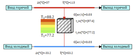
Figure 2. Heat exchanger cell model.
The model of the tubular heat exchanger is easily adjustable. You can change just one parameter – the number of sections along the pipe length and observe the calculation results at different divisions. We will calculate several options, starting with a division into 5 points along the length (Fig. 3) and up to 100 points along the length (Fig. 4).
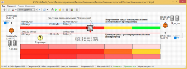
Figure 3. Steady-state temperature distribution with 5 calculation points.
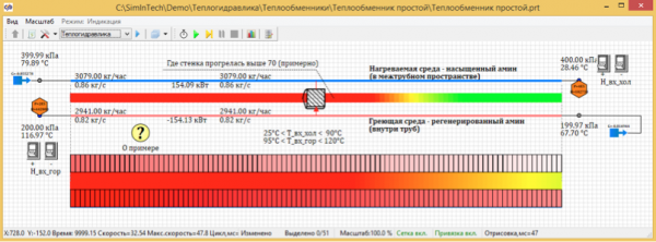
Figure 4. Steady-state temperature distribution with 100 calculation points.
As a result of the calculations, it was found that the steady-state temperature with a division into 100 points is 67.7 degrees. With a division into 5 calculation points, the temperature is 72.66 degrees Celsius.
Additionally, the calculation speed relative to real-time is displayed at the bottom of the window.
Let's see how the steady-state temperature and calculation speed change depending on the number of calculation points. The difference in steady-state temperatures for calculations with different numbers of calculation cells can be used to assess the accuracy of the obtained result.
Table 1. Dependence of temperature and calculation speed on the number of calculation points along the length of the heat exchanger.
| Number of calculation points | Steady-state temperature | Calculation speed |
| 5 | 72,66 | 426 |
| 10 | 70.19 | 194 |
| 25 | 68.56 | 124 |
| 50 | 67.99 | 66 |
| 100 | 67.8 | 32 |
Analyzing this table, we can draw the following conclusions:
- The calculation speed decreases proportionally to the number of calculation points in the heat exchanger model.
- The change in calculation accuracy occurs exponentially. With an increase in the number of points, the refinement at each subsequent increase decreases.
In the case of a plate heat exchanger with cross-flow of the heat carrier, as shown in Fig. 1, creating an equivalent model from elementary calculation cells becomes slightly more complicated. We need to connect the cells in such a way as to organize cross flow. For 4 cells, the scheme will look as shown in Fig. 5.
The flow of the coolant is divided into hot and cold branches into two channels, which will connect through heat structures, allowing the coolant to exchange heat with different channels as it flows through. In simulating the cross flow, the hot coolant travels from left to right (see Fig. 5) in each channel, sequentially exchanging heat with the cold coolant, which moves from bottom to top (see Fig. 5). The hottest point is in the upper left corner, as the hot coolant exchanges heat with the already heated coolant from the cold channel. The coldest point is in the lower right, where the cold coolant exchanges heat with the hot coolant that has already cooled down in the first section.
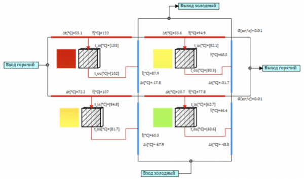
Figure 5. Cross-flow model with 4 calculation cells.
Such a model for a plate heat exchanger does not account for heat transfer between cells due to thermal conductivity and neglects the mixing of the coolant, as each channel is isolated.
However, in our case, this last limitation does not reduce accuracy since the heat exchanger design includes a corrugated membrane that separates the flow into numerous isolated channels for the coolant (see Fig. 1). Let's examine how the calculation accuracy is affected when modeling a plate heat exchanger with an increased number of calculation cells.
For accuracy analysis, we use two options for dividing the heat exchanger into calculation cells:
- Each square cell contains two hydraulic elements (cold and hot flows) and one thermal element. (see Fig. 5)
- Each square cell contains six hydraulic elements (three sections in hot and cold flows) and three thermal elements.
In the latter case, we use two types of connections:
- counter-flow of cold and hot streams;
- co-current flow of cold and hot streams.
Counter-flow increases efficiency compared to cross flow, while co-current flow reduces it. With a large number of cells, averaging occurs in the flow, bringing it closer to actual cross-flow conditions (see Fig. 6).
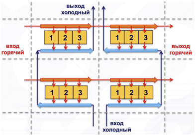
Figure 6. Cross-flow model with four cells, each containing three elements.
Figure 7 shows the results of the steady-state temperature distribution in the heat exchanger when air at a temperature of 150 °C is supplied through the hot line, and 21 °C through the cold line, for various model partitioning options. The color and numbers in the cell reflect the average wall temperature in the calculated cell.
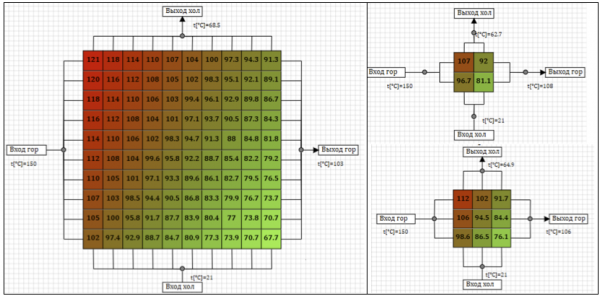
Figure 7. Steady-state temperatures for different calculation schemes.
Table 2 presents the steady-state temperature of the heated air after the heat exchanger depending on the partitioning of the heat exchanger model into cells.
Table 2. Dependency of temperature on the number of calculation cells in the heat exchanger.
| Model dimensions | Steady-state temperature 1 element in the cell | Steady-state temperature 3 elements in the cell |
| 2x2 | 62,7 | 67.7 |
| 3×3 | 64.9 | 68.5 |
| 4x4 | 66.2 | 68.9 |
| 8x8 | 68.1 | 69.5 |
| 10×10 | 68.5 | 69.7 |
| 20×20 | 69.4 | 69.9 |
| 40×40 | 69.8 | 70.1 |
As the number of calculation cells in the model increases, the final steady-state temperature rises. The difference between the steady-state temperature for different partitions can be considered an indicator of calculation accuracy. It is evident that as the number of calculation cells increases, the temperature approaches a limit, and the increase in accuracy is not proportional to the number of calculation points.
The question arises, what accuracy of the model do we need?
The answer to this question depends on the purpose of our model. Since this article discusses model-oriented design, we create the model for tuning the control system. This means that the accuracy of the model should be comparable to the accuracy of the sensors used in the system.
In our case, the temperature is measured by a thermocouple with an accuracy of ±2.5 °C. Any accuracy higher for the purposes of tuning the control system is useless; our actual control system simply will not 'see' it. Thus, if we assume that the limit temperature with an infinite number of partitions is 70 °C, a sufficient accuracy would be a model that gives us more than 67.5 °C. All models with 3 points in the calculation cell and models larger than 5x5 with one point in the cell. (Highlighted in green in Table 2)
Dynamic operating modes
To assess the dynamic mode, we will evaluate the temperature change process at the hottest and coldest points on the wall of the heat exchanger for different calculation scheme options. (see Fig. 8)
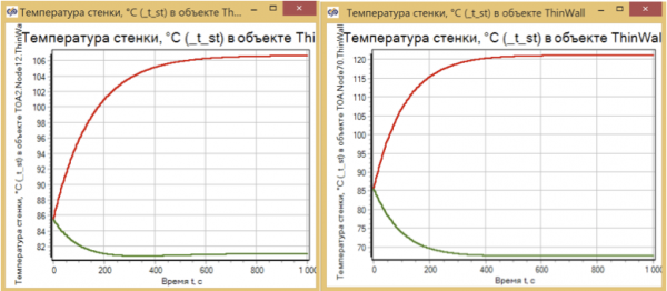
Figure 8. Heating of the heat exchanger. Models of dimensions 2x2 and 10x10.
It is clear that the duration and nature of the transition process are virtually independent of the number of computational cells and are determined solely by the mass of the heated metal.
Thus, we conclude that for accurate modeling of the heat exchanger in the temperature range of 20 to 150 °C, with the precision required by the control system, approximately 10 to 20 calculation points are sufficient.
Calibration of the dynamic model based on experiments
Having a mathematical model, as well as experimental data from the heat exchanger purging, we only need to make a simple correction by introducing an intensification coefficient into the model so that the calculations match the experimental results.
Moreover, using a graphical environment for model creation, we can do this automatically. Figure 9 shows the algorithm for selecting the intensification coefficients for heat exchange. Experimental data is fed into the input, the heat exchanger model is connected, and the necessary coefficients for each mode are obtained as output.
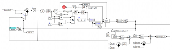
Figure 9. Algorithm for selecting the intensification coefficient based on experimental results.
Thus, we determine the very coefficient for the Nusselt number and eliminate uncertainty in the calculation formulas. For various operating modes and temperatures, the values of the correction coefficients may vary; however, for similar operating modes (normal operation), they turn out to be quite close. For example, for this heat exchanger, the coefficient ranges from 0.492 to 0.655 for different modes.
If we apply a coefficient of 0.6, then in the investigated operating modes, the calculation error will be less than the error of the thermocouple, thus for the control system, the mathematical model of the heat exchanger will be fully adequate to the actual model.
Results of heat exchanger model calibration
To assess the quality of heat exchange, a special characteristic is used – efficiency:
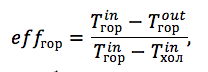
where:
effhot – efficiency of the heat exchanger for the hot heat carrier;
Thotin – temperature at the inlet of the heat exchanger along the path of the hot heat carrier;
Thotout – temperature at the outlet of the heat exchanger along the path of the hot heat carrier;
Tcoldin – the temperature at the inlet of the heat exchanger in the cold heat carrier flow path.
Table 3 contains the values of the deviation of the heat exchanger model's efficiency from the experimental results at various flow rates in the hot and cold lines.
Table 3. Calculation errors of heat exchange efficiency in %.
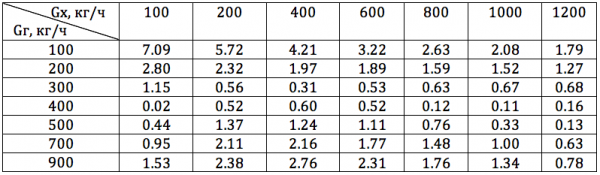
In our case, the selected coefficient can be used in all operating modes of interest. If at low flow rates, where the error is greater, the necessary accuracy is not achieved, we can use a variable intensification coefficient that will depend on the current flow rate.
For example, in Figure 10, the intensification coefficient is calculated according to a specified formula depending on the current flow rate in the channel cells.
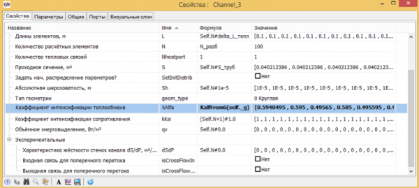
Figure 10. Variable intensification coefficient of heat exchange.
Conclusions
- Understanding physical laws allows for the creation of dynamic models of objects for model-oriented design.
- The model must be verified and calibrated based on test data.
- Model development tools should allow the developer to adjust the model based on test results.
- Use the correct model-oriented approach and happiness will follow!
A bonus for those who read to the end.
Only registered users can participate in the survey. , please.
What else should we talk about?
76,2%How to prove that the program in the model corresponds to the program in the hardware.
23,8%How to use computations on a Supercomputer for model-oriented design.
21 users voted. 1 user abstained.
Source: habr.com
