Solving the equation of simple linear regression

This article discusses several methods for determining the mathematical equation of a simple (pair) regression line.

All the methods presented here for solving the equation are based on the least squares method. We will denote the methods as follows:

• Analytical solution
• Gradient descent
• Stochastic gradient descent

For each method of solving the line equation, various functions are provided in the article, which are mainly divided into those that are written without using the library NumPy and those that use NumPy. It is believed that skillful use of NumPy will reduce computational costs.

All the code presented in the article is written in the python 2.7 using Jupyter Notebook. The source code and the data sample file are posted on GitHub

The article is primarily oriented towards both beginners and those who have just started to delve into the vast field of artificial intelligence — machine learning.

To illustrate the material, we will use a very simple example.

Conditions of the example

We have five values that characterize the dependency Y from X (Table No. 1):

Table No. 1 "Conditions of the Example"

Let’s assume that the values — are the months of the year, and — the revenue for that month. In other words, revenue depends on the month of the year, and — is the only feature from which revenue depends.

The example is rather mediocre, both in terms of the conditional dependency of revenue on the month of the year, as well as in terms of the number of values — there are very few. However, such simplification will help to explain, in layman’s terms, material that isn't always easily grasped by beginners. Additionally, the simplicity of the numbers will allow those interested to solve the example on "paper" without significant labor costs.

Let’s assume that the given dependency in the example can be quite well approximated by the mathematical equation of a simple (pair) regression line of the form:

where — is the month in which the revenue was received, — the revenue corresponding to the month, and — the coefficients of the estimated line.

Note that the coefficient is often referred to as the slope coefficient or the gradient of the estimated line; it represents the amount by which will change with variation .

It is clear that our task in this example is to select coefficients in the equation and , under which the deviations of our calculated revenue values by month from the true answers, i.e., the values provided in the sample, will be minimal.

The method of least squares

According to the least squares method, deviations should be calculated by squaring them. This approach avoids mutual cancellation of deviations when they have opposite signs. For example, if in one case, the deviation is +5 (plus five), and in another -5 (minus five), then the sum of the deviations will cancel each other out and amount to 0 (zero). It is also possible not to square the deviation but to use the modulus property, in which case all deviations will be positive and will accumulate. We will not dwell on this point in detail but will simply note that for convenience in calculations, it is customary to square the deviation.

This is what the formula looks like, with the help of which we will determine the smallest sum of squared deviations (errors):

where — this is the function that approximates the true answers (i.e., the revenue we calculated),

— these are the true answers (the revenue provided in the sample),

— this is the sample index (the month number in which the deviation is being determined)

We will differentiate the function, determine the equations of the partial derivatives, and be ready to move on to analytical solutions. But first, let's take a little detour about what differentiation is and recall the geometric meaning of a derivative.

Differentiation

Differentiation is the operation of finding the derivative of a function.

What is the derivative needed for? The derivative of a function characterizes the rate of change of the function and indicates its direction. If the derivative at a given point is positive, then the function is increasing; otherwise, the function is decreasing. And the greater the absolute value of the derivative, the higher the rate of change of the function values, as well as the steeper the slope of the function's graph.

For example, in a Cartesian coordinate system, the value of the derivative at point M(0,0) equal to +25 means that at the given point, when shifting the value to the right by a conditional unit, the value increases by 25 conditional units. On the graph, this appears as a fairly steep angle of ascent in values. from the specified point.

Another example. The value of the derivative equal to -0,1 means that with a shift of by one conditional unit, the value decreases by only 0.1 conditional units. Meanwhile, on the function's graph, we can observe a barely noticeable downward slope. Drawing an analogy with a mountain, it feels like we are slowly descending a gentle slope, unlike the previous example where we had to take very steep peaks :)

Thus, by differentiating the function with respect to the coefficients and , we will determine the equations of the first-order partial derivatives. After determining the equations, we will obtain a system of two equations, and by solving them, we can find such values of the coefficients and , under which the values of the corresponding derivatives at the specified points change by very, very small amounts, while in the case of the analytical solution they do not change at all. In other words, the error function with the found coefficients will reach a minimum, since the values of the partial derivatives at these points will be zero.

So, according to the differentiation rules, the equation of the first-order partial derivative with respect to the coefficient will take the form:

the equation of the first-order partial derivative with respect to will take the form:

As a result, we obtained a system of equations that has a quite simple analytical solution:

begin{equation*}
begin{cases}
na + bsumlimits_{i=1}^nx_i — sumlimits_{i=1}^ny_i = 0

sumlimits_{i=1}^nx_i(a + bsumlimits_{i=1}^nx_i — sumlimits_{i=1}^ny_i) = 0
end{cases}
end{equation*}

Before solving the equation, we will first load, check the correctness of the loading, and format the data.

Loading and formatting data

It should be noted that due to the fact that for the analytical solution, and later for gradient and stochastic gradient descent, we will apply the code in two variations: using the library NumPy and without it, we will need appropriate data formatting (see code).

Data loading and processing code

# импортируем все нужные нам библиотеки
import pandas as pd
import numpy as np
import matplotlib.pyplot as plt
import math
import pylab as pl
import random

# графики отобразим в Jupyter
%matplotlib inline

# укажем размер графиков
from pylab import rcParams
rcParams['figure.figsize'] = 12, 6

# отключим предупреждения Anaconda
import warnings
warnings.simplefilter('ignore')

# загрузим значения
table_zero = pd.read_csv('data_example.txt', header=0, sep='t')

# посмотрим информацию о таблице и на саму таблицу
print table_zero.info()
print '********************************************'
print table_zero
print '********************************************'

# подготовим данные без использования NumPy

x_us = []
[x_us.append(float(i)) for i in table_zero['x']]
print x_us
print type(x_us)
print '********************************************'

y_us = []
[y_us.append(float(i)) for i in table_zero['y']]
print y_us
print type(y_us)
print '********************************************'

# подготовим данные с использованием NumPy

x_np = table_zero[['x']].values
print x_np
print type(x_np)
print x_np.shape
print '********************************************'

y_np = table_zero[['y']].values
print y_np
print type(y_np)
print y_np.shape
print '********************************************'

Visualization

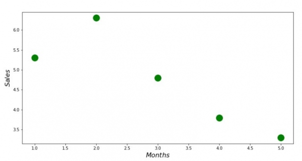
Now, after we have first loaded the data, second checked the correctness of the loading, and finally formatted the data, let's proceed to the first visualization. Often, the method used for this is pairplot a library Seaborn. In our example, due to the limited digits, it makes no sense to use a library Seaborn. We will use a regular library Matplotlib and will only look at the scatter plot.

Scatter plot code

print 'Chart №1 "Dependency of revenue on the month of the year"'

plt.plot(x_us,y_us,'o',color='green',markersize=16)
plt.xlabel('$Months$', size=16)
plt.ylabel('$Sales$', size=16)
plt.show()

Chart №1 «Dependency of revenue on the month of the year»

Analytical solution

We will use the most ordinary tools in python and solve the system of equations:

begin{equation*}
begin{cases}
na + bsumlimits_{i=1}^nx_i — sumlimits_{i=1}^ny_i = 0

sumlimits_{i=1}^nx_i(a + bsumlimits_{i=1}^nx_i — sumlimits_{i=1}^ny_i) = 0
end{cases}
end{equation*}

By Cramer's rule we will find the overall determinant, as well as the determinants for and for , after which, by dividing the determinant for by the overall determinant — we will find the coefficient , similarly we will find the coefficient .

Analytical solution code

# определим функцию для расчета коэффициентов a и b по правилу Крамера
def Kramer_method (x,y):
        # сумма значений (все месяца)
    sx = sum(x)
        # сумма истинных ответов (выручка за весь период)
    sy = sum(y)
        # сумма произведения значений на истинные ответы
    list_xy = []
    [list_xy.append(x[i]*y[i]) for i in range(len(x))]
    sxy = sum(list_xy)
        # сумма квадратов значений
    list_x_sq = []
    [list_x_sq.append(x[i]**2) for i in range(len(x))]
    sx_sq = sum(list_x_sq)
        # количество значений
    n = len(x)
        # общий определитель
    det = sx_sq*n - sx*sx
        # определитель по a
    det_a = sx_sq*sy - sx*sxy
        # искомый параметр a
    a = (det_a / det)
        # определитель по b
    det_b = sxy*n - sy*sx
        # искомый параметр b
    b = (det_b / det)
        # контрольные значения (прооверка)
    check1 = (n*b + a*sx - sy)
    check2 = (b*sx + a*sx_sq - sxy)
    return [round(a,4), round(b,4)]

# запустим функцию и запишем правильные ответы
ab_us = Kramer_method(x_us,y_us)
a_us = ab_us[0]
b_us = ab_us[1]
print ' 33[1m' + ' 33[4m' + "Оптимальные значения коэффициентов a и b:"  + ' 33[0m' 
print 'a =', a_us
print 'b =', b_us
print

# определим функцию для подсчета суммы квадратов ошибок
def errors_sq_Kramer_method(answers,x,y):
    list_errors_sq = []
    for i in range(len(x)):
        err = (answers[0] + answers[1]*x[i] - y[i])**2
        list_errors_sq.append(err)
    return sum(list_errors_sq)

# запустим функцию и запишем значение ошибки
error_sq = errors_sq_Kramer_method(ab_us,x_us,y_us)
print ' 33[1m' + ' 33[4m' + "Сумма квадратов отклонений" + ' 33[0m'
print error_sq
print

# замерим время расчета
# print ' 33[1m' + ' 33[4m' + "Время выполнения расчета суммы квадратов отклонений:" + ' 33[0m'
# % timeit error_sq = errors_sq_Kramer_method(ab,x_us,y_us)

Here is what we got:

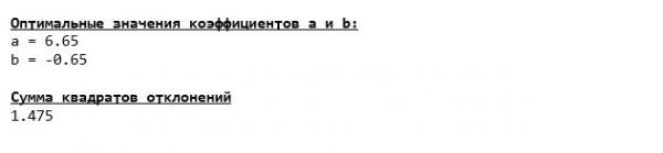
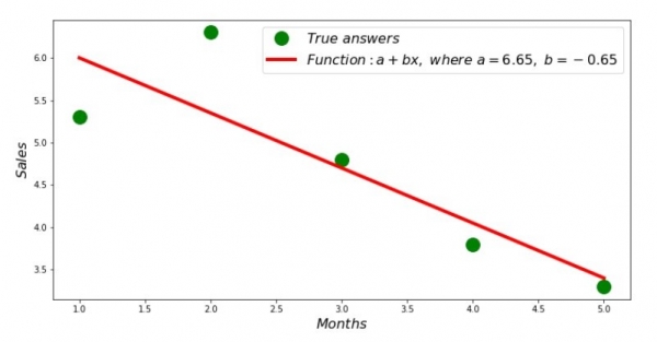
So, the values of the coefficients are found, and the sum of squares of deviations is established. Let's draw a line on the scatter histogram according to the found coefficients.

Regression line code

# определим функцию для формирования массива рассчетных значений выручки
def sales_count(ab,x,y):
    line_answers = []
    [line_answers.append(ab[0]+ab[1]*x[i]) for i in range(len(x))]
    return line_answers

# построим графики
print 'Грфик№2 "Правильные и расчетные ответы"'
plt.plot(x_us,y_us,'o',color='green',markersize=16, label = '$True$ $answers$')
plt.plot(x_us, sales_count(ab_us,x_us,y_us), color='red',lw=4,
         label='$Function: a + bx,$ $where$ $a='+str(round(ab_us[0],2))+',$ $b='+str(round(ab_us[1],2))+'$')
plt.xlabel('$Months$', size=16)
plt.ylabel('$Sales$', size=16)
plt.legend(loc=1, prop={'size': 16})
plt.show()

Chart №2 «Actual and calculated answers»

We can look at the deviation chart for each month. In our case, we won't derive any significant practical value from it, but we will satisfy our curiosity about how well the equation of simple linear regression characterizes the dependence of revenue on the month of the year.

Deviation chart code

# определим функцию для формирования массива отклонений в процентах
def error_per_month(ab,x,y):
    sales_c = sales_count(ab,x,y)
    errors_percent = []
    for i in range(len(x)):
        errors_percent.append(100*(sales_c[i]-y[i])/y[i])
    return errors_percent

# построим график
print 'График№3 "Отклонения по-месячно, %"'
plt.gca().bar(x_us, error_per_month(ab_us,x_us,y_us), color='brown')
plt.xlabel('Months', size=16)
plt.ylabel('Calculation error, %', size=16)
plt.show()

Chart №3 «Deviations, %»

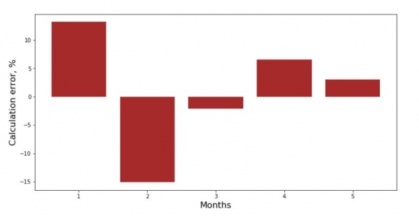
Not perfect, but we have completed our task.

Let's write a function that determines the coefficients and uses the library NumPy, specifically — we will write two functions: one using the pseudo-inverse matrix (not recommended in practice, as the computation process is complex and unstable), the other using the matrix equation.

Analytical solution code (NumPy)

# для начала добавим столбец с не изменяющимся значением в 1. 
# Данный столбец нужен для того, чтобы не обрабатывать отдельно коэффицент a
vector_1 = np.ones((x_np.shape[0],1))
x_np = table_zero[['x']].values # на всякий случай приведем в первичный формат вектор x_np
x_np = np.hstack((vector_1,x_np))

# проверим то, что все сделали правильно
print vector_1[0:3]
print x_np[0:3]
print '***************************************'
print

# напишем функцию, которая определяет значения коэффициентов a и b с использованием псевдообратной матрицы
def pseudoinverse_matrix(X, y):
    # задаем явный формат матрицы признаков
    X = np.matrix(X)
    # определяем транспонированную матрицу
    XT = X.T
    # определяем квадратную матрицу
    XTX = XT*X
    # определяем псевдообратную матрицу
    inv = np.linalg.pinv(XTX)
    # задаем явный формат матрицы ответов
    y = np.matrix(y)
    # находим вектор весов
    return (inv*XT)*y

# запустим функцию
ab_np = pseudoinverse_matrix(x_np, y_np)
print ab_np
print '***************************************'
print

# напишем функцию, которая использует для решения матричное уравнение
def matrix_equation(X,y):
    a = np.dot(X.T, X)
    b = np.dot(X.T, y)
    return np.linalg.solve(a, b)

# запустим функцию
ab_np = matrix_equation(x_np,y_np)
print ab_np

Let's compare the time spent determining the coefficients and , according to the 3 presented methods.

Code to calculate calculation time

print ' 33[1m' + ' 33[4m' + "Time taken to calculate coefficients without using the NumPy library:" + ' 33[0m'
% timeit ab_us = Kramer_method(x_us,y_us)
print '***************************************'
print
print ' 33[1m' + ' 33[4m' + "Time taken to calculate coefficients using the pseudo-inverse matrix:" + ' 33[0m'
%timeit ab_np = pseudoinverse_matrix(x_np, y_np)
print '***************************************'
print
print ' 33[1m' + ' 33[4m' + "Time taken to calculate coefficients using the matrix equation:" + ' 33[0m'
%timeit ab_np = matrix_equation(x_np, y_np)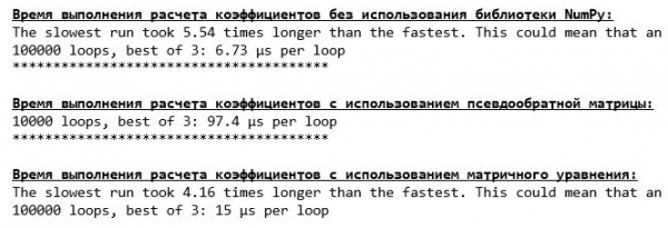

With a small amount of data, the 'custom' function takes the lead, finding coefficients using Cramer's method.

Now we can move on to other methods of finding coefficients. and .

Gradient descent

Let's start by defining what a gradient is. Simply put, a gradient is a segment that indicates the direction of the maximum growth of a function. Analogous to climbing a mountain, where the gradient points to the steepest ascent to the peak. Expanding on the mountain example, we recall that what we actually need is the steepest descent to reach the valley, or the minimum — a point where the function neither increases nor decreases. At this point, the derivative will be zero. Therefore, we need not a gradient, but an anti-gradient. To find the anti-gradient, we just multiply the gradient by -1 (minus one).

Note that a function can have multiple minima, and having descended into one of them using the proposed algorithm, we may not find another minimum that could be lower than the one found. Relax, this is not a concern for us! In our case, we are dealing with a single minimum, as our function on the graph is simply a parabola. And as we should all know from school mathematics, a parabola has only one minimum.

After we have determined the purpose of the gradient, and knowing that the gradient is a segment, meaning a vector with specified coordinates, which are exactly those coefficients and we can implement gradient descent.

Before we begin, I suggest reading just a few sentences about the descent algorithm:

• We define the coefficients' coordinates in a pseudo-random manner. and In our example, we will define the coefficients near zero. This is common practice, but each case may have its own specific approach.
• From the coordinate we subtract the value of the first-order partial derivative at the point. Thus, if the derivative is positive, the function is increasing. Consequently, by subtracting the value of the derivative, we move in the opposite direction of growth, that is, towards descent. If the derivative is negative, then the function is decreasing at this point, and by subtracting the value of the derivative, we move towards descent.
• We perform a similar operation with the coordinate : we subtract the value of the partial derivative at the point .
• To avoid skipping the minimum and flying into deep space, it is necessary to set the step size towards descent. In general, a whole article could be written about how to properly set the step size and how to change it during descent to reduce computational costs. But now we have a slightly different task, and through the scientific method of 'trial and error'—or as it's commonly said, empirically—we will determine the step size.
• After we have subtracted the derivative values from the given coordinates and we obtain new coordinates and . We take the next step (subtraction) from the already calculated coordinates. And thus, the cycle restarts over and over again until the required convergence is achieved.

That's it! Now we are ready to embark on a quest for the deepest part of the Mariana Trench. Let's begin.

Code for gradient descent

# напишем функцию градиентного спуска без использования библиотеки NumPy. 
# Функция на вход принимает диапазоны значений x,y, длину шага (по умолчанию=0,1), допустимую погрешность(tolerance)
def gradient_descent_usual(x_us,y_us,l=0.1,tolerance=0.000000000001):
    # сумма значений (все месяца)
    sx = sum(x_us)
    # сумма истинных ответов (выручка за весь период)
    sy = sum(y_us)
    # сумма произведения значений на истинные ответы
    list_xy = []
    [list_xy.append(x_us[i]*y_us[i]) for i in range(len(x_us))]
    sxy = sum(list_xy)
    # сумма квадратов значений
    list_x_sq = []
    [list_x_sq.append(x_us[i]**2) for i in range(len(x_us))]
    sx_sq = sum(list_x_sq)
    # количество значений
    num = len(x_us)
    # начальные значения коэффициентов, определенные псевдослучайным образом
    a = float(random.uniform(-0.5, 0.5))
    b = float(random.uniform(-0.5, 0.5))
    # создаем массив с ошибками, для старта используем значения 1 и 0
    # после завершения спуска стартовые значения удалим
    errors = [1,0]
    # запускаем цикл спуска
    # цикл работает до тех пор, пока отклонение последней ошибки суммы квадратов от предыдущей, не будет меньше tolerance
    while abs(errors[-1]-errors[-2]) > tolerance:
        a_step = a - l*(num*a + b*sx - sy)/num
        b_step = b - l*(a*sx + b*sx_sq - sxy)/num
        a = a_step
        b = b_step
        ab = [a,b]
        errors.append(errors_sq_Kramer_method(ab,x_us,y_us))
    return (ab),(errors[2:])

# запишем массив значений 
list_parametres_gradient_descence = gradient_descent_usual(x_us,y_us,l=0.1,tolerance=0.000000000001)


print ' 33[1m' + ' 33[4m' + "Значения коэффициентов a и b:" + ' 33[0m'
print 'a =', round(list_parametres_gradient_descence[0][0],3)
print 'b =', round(list_parametres_gradient_descence[0][1],3)
print


print ' 33[1m' + ' 33[4m' + "Сумма квадратов отклонений:" + ' 33[0m'
print round(list_parametres_gradient_descence[1][-1],3)
print



print ' 33[1m' + ' 33[4m' + "Количество итераций в градиентном спуске:" + ' 33[0m'
print len(list_parametres_gradient_descence[1])
print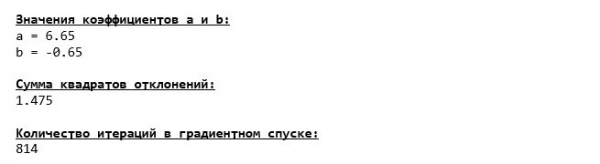

We have descended to the very bottom of the Mariana Trench and found all the same coefficient values and , which was to be expected.

Let’s make one more dive, but this time our deep-sea apparatus will utilize different technologies, namely the library NumPy.

Code for gradient descent (NumPy)

# перед тем определить функцию для градиентного спуска с использованием библиотеки NumPy, 
# напишем функцию определения суммы квадратов отклонений также с использованием NumPy
def error_square_numpy(ab,x_np,y_np):
    y_pred = np.dot(x_np,ab)
    error = y_pred - y_np
    return sum((error)**2)

# напишем функцию градиентного спуска с использованием библиотеки NumPy. 
# Функция на вход принимает диапазоны значений x,y, длину шага (по умолчанию=0,1), допустимую погрешность(tolerance)
def gradient_descent_numpy(x_np,y_np,l=0.1,tolerance=0.000000000001):
    # сумма значений (все месяца)
    sx = float(sum(x_np[:,1]))
    # сумма истинных ответов (выручка за весь период)
    sy = float(sum(y_np))
    # сумма произведения значений на истинные ответы
    sxy = x_np*y_np
    sxy = float(sum(sxy[:,1]))
    # сумма квадратов значений
    sx_sq = float(sum(x_np[:,1]**2))
    # количество значений
    num = float(x_np.shape[0])
    # начальные значения коэффициентов, определенные псевдослучайным образом
    a = float(random.uniform(-0.5, 0.5))
    b = float(random.uniform(-0.5, 0.5))
    # создаем массив с ошибками, для старта используем значения 1 и 0
    # после завершения спуска стартовые значения удалим
    errors = [1,0]
    # запускаем цикл спуска
    # цикл работает до тех пор, пока отклонение последней ошибки суммы квадратов от предыдущей, не будет меньше tolerance
    while abs(errors[-1]-errors[-2]) > tolerance:
        a_step = a - l*(num*a + b*sx - sy)/num
        b_step = b - l*(a*sx + b*sx_sq - sxy)/num
        a = a_step
        b = b_step
        ab = np.array([[a],[b]])
        errors.append(error_square_numpy(ab,x_np,y_np))
    return (ab),(errors[2:])

# запишем массив значений 
list_parametres_gradient_descence = gradient_descent_numpy(x_np,y_np,l=0.1,tolerance=0.000000000001)

print ' 33[1m' + ' 33[4m' + "Значения коэффициентов a и b:" + ' 33[0m'
print 'a =', round(list_parametres_gradient_descence[0][0],3)
print 'b =', round(list_parametres_gradient_descence[0][1],3)
print


print ' 33[1m' + ' 33[4m' + "Сумма квадратов отклонений:" + ' 33[0m'
print round(list_parametres_gradient_descence[1][-1],3)
print

print ' 33[1m' + ' 33[4m' + "Количество итераций в градиентном спуске:" + ' 33[0m'
print len(list_parametres_gradient_descence[1])
print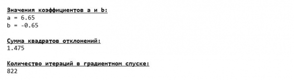

The coefficient values and are unchanged.

Let’s examine how the error changed during gradient descent, specifically how the sum of squared deviations varied with each step.

Code for the plot of the sum of squared deviations

print 'Plot #4 "Sum of squared deviations by step"'
plt.plot(range(len(list_parametres_gradient_descence[1])), list_parametres_gradient_descence[1], color='red', lw=3)
plt.xlabel('Steps (Iteration)', size=16)
plt.ylabel('Sum of squared deviations', size=16)
plt.show()

Plot #4 "Sum of squared deviations during gradient descent"

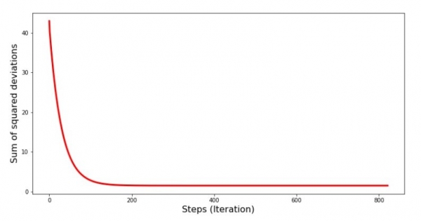
In the plot, we see that with each step the error decreases, and after a certain number of iterations, we observe an almost horizontal line.

Finally, let’s assess the difference in execution time of the code:

Code to determine the computation time of gradient descent

print ' 33[1m' + ' 33[4m' + "Execution time of gradient descent without using the NumPy library:" + ' 33[0m'
%timeit list_parametres_gradient_descence = gradient_descent_usual(x_us,y_us,l=0.1,tolerance=0.000000000001)
print '***************************************'
print

print ' 33[1m' + ' 33[4m' + "Execution time of gradient descent using the NumPy library:" + ' 33[0m'
%timeit list_parametres_gradient_descence = gradient_descent_numpy(x_np,y_np,l=0.1,tolerance=0.000000000001)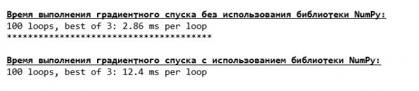

Perhaps we are doing something wrong, but again, a simple 'homemade' function that does not use a library NumPy outperforms the execution time of the function that uses the library NumPy.

But we are not standing still, we are moving towards exploring yet another exciting way to solve the equation of simple linear regression. Meet!

Stochastic gradient descent

To better understand the principle of stochastic gradient descent, it helps to define its differences from ordinary gradient descent. In the case of gradient descent, in the derivative equations of and we used the sums of the values of all features and the true responses available in the sample (that is, the sums of all and ). In stochastic gradient descent, we will not use all the values available in the sample, but instead, we will pseudorandomly select a so-called sample index and use its values.

For example, if the index is determined as number 3 (three), then we take the values and , then we substitute the values into the derivative equations and determine new coordinates. Next, having determined the coordinates, we again pseudorandomly determine the sample index, substitute the values corresponding to the index into the partial derivative equations, and redefine the coordinates and and so on until convergence is achieved. At first glance, it may seem like how this could possibly work; however, it does work. It is worth noting that the error does not decrease with every step, but the trend is undoubtedly present.

What are the advantages of stochastic gradient descent over regular gradient descent? When the sample size is very large, measured in tens of thousands of values, it is much easier to process, say, a random thousand of them than the entire sample. This is when stochastic gradient descent comes into play. In our case, we will not notice a big difference.

Let's take a look at the code.

Code for stochastic gradient descent

# определим функцию стох.град.шага
def stoch_grad_step_usual(vector_init, x_us, ind, y_us, l):
#     выбираем значение икс, которое соответствует случайному значению параметра ind 
# (см.ф-цию stoch_grad_descent_usual)
    x = x_us[ind]
#     рассчитывыаем значение y (выручку), которая соответствует выбранному значению x
    y_pred = vector_init[0] + vector_init[1]*x_us[ind]
#     вычисляем ошибку расчетной выручки относительно представленной в выборке
    error = y_pred - y_us[ind]
#     определяем первую координату градиента ab
    grad_a = error
#     определяем вторую координату ab
    grad_b = x_us[ind]*error
#     вычисляем новый вектор коэффициентов
    vector_new = [vector_init[0]-l*grad_a, vector_init[1]-l*grad_b]
    return vector_new


# определим функцию стох.град.спуска
def stoch_grad_descent_usual(x_us, y_us, l=0.1, steps = 800):
#     для самого начала работы функции зададим начальные значения коэффициентов
    vector_init = [float(random.uniform(-0.5, 0.5)), float(random.uniform(-0.5, 0.5))]
    errors = []
#     запустим цикл спуска
# цикл расчитан на определенное количество шагов (steps)
    for i in range(steps):
        ind = random.choice(range(len(x_us)))
        new_vector = stoch_grad_step_usual(vector_init, x_us, ind, y_us, l)
        vector_init = new_vector
        errors.append(errors_sq_Kramer_method(vector_init,x_us,y_us))
    return (vector_init),(errors)


# запишем массив значений 
list_parametres_stoch_gradient_descence = stoch_grad_descent_usual(x_us, y_us, l=0.1, steps = 800)

print ' 33[1m' + ' 33[4m' + "Значения коэффициентов a и b:" + ' 33[0m'
print 'a =', round(list_parametres_stoch_gradient_descence[0][0],3)
print 'b =', round(list_parametres_stoch_gradient_descence[0][1],3)
print


print ' 33[1m' + ' 33[4m' + "Сумма квадратов отклонений:" + ' 33[0m'
print round(list_parametres_stoch_gradient_descence[1][-1],3)
print

print ' 33[1m' + ' 33[4m' + "Количество итераций в стохастическом градиентном спуске:" + ' 33[0m'
print len(list_parametres_stoch_gradient_descence[1])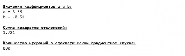

We look closely at the coefficients and catch ourselves asking, 'How is this possible?'. We have obtained different coefficient values. and Could it be that stochastic gradient descent found more optimal parameters for the equation? Unfortunately, no. Just look at the sum of squared deviations and see that with the new coefficient values, the error increases. Let's not rush to despair. We will build a graph to illustrate the change in error.

Code for the graph of the sum of squared deviations during stochastic gradient descent

print 'Graph #5 "Sum of squared deviations step by step"'
plt.plot(range(len(list_parametres_stoch_gradient_descence[1])), list_parametres_stoch_gradient_descence[1], color='red', lw=2)
plt.xlabel('Steps (Iteration)', size=16)
plt.ylabel('Sum of squared deviations', size=16)
plt.show()

Graph #5 "Sum of squared deviations during stochastic gradient descent"

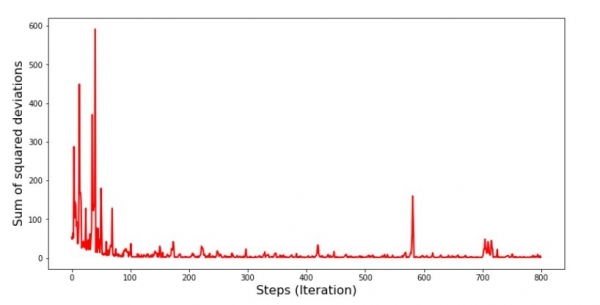
Looking at the graph, everything falls into place, and now we will fix everything.

So, what happened? The following occurred. When we randomly select a month, our algorithm aims to reduce the error in revenue calculation specifically for that month. We then choose another month and repeat the calculation, but now we are reducing the error for the second selected month. And let’s remember that our first two months significantly deviate from the line of the simple linear regression equation. This means that when either of these two months is chosen, reducing the error for each of them seriously increases the error across the entire sample. So what should we do? The answer is simple: we need to reduce the descent step. By decreasing the descent step, the error will also stop 'jumping' up and down. Well, the error won’t stop jumping, but it will do so less briskly :) Let’s check.

Code to run SGD with a smaller step

# запустим функцию, уменьшив шаг в 100 раз и увеличив количество шагов соответсвующе 
list_parametres_stoch_gradient_descence = stoch_grad_descent_usual(x_us, y_us, l=0.001, steps = 80000)

print ' 33[1m' + ' 33[4m' + "Значения коэффициентов a и b:" + ' 33[0m'
print 'a =', round(list_parametres_stoch_gradient_descence[0][0],3)
print 'b =', round(list_parametres_stoch_gradient_descence[0][1],3)
print


print ' 33[1m' + ' 33[4m' + "Сумма квадратов отклонений:" + ' 33[0m'
print round(list_parametres_stoch_gradient_descence[1][-1],3)
print



print ' 33[1m' + ' 33[4m' + "Количество итераций в стохастическом градиентном спуске:" + ' 33[0m'
print len(list_parametres_stoch_gradient_descence[1])

print 'График №6 "Сумма квадратов отклонений по-шагово"'
plt.plot(range(len(list_parametres_stoch_gradient_descence[1])), list_parametres_stoch_gradient_descence[1], color='red', lw=2)
plt.xlabel('Steps (Iteration)', size=16)
plt.ylabel('Sum of squared deviations', size=16)
plt.show()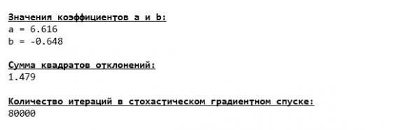

Graph #6 "Sum of squared deviations during stochastic gradient descent (80,000 steps)"

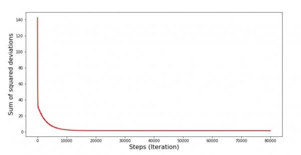
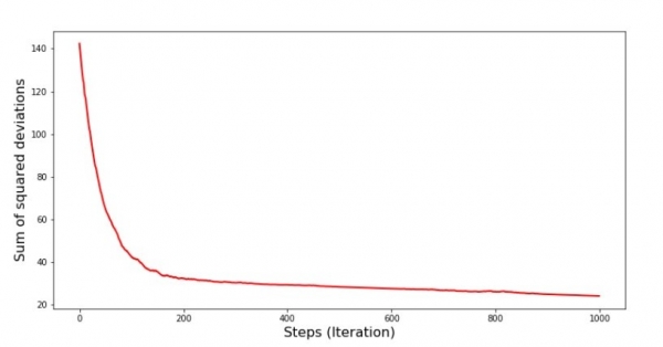
The coefficient values have improved, but they are still not ideal. Hypothetically, this could be addressed in the following way. We select, for example, the coefficient values from the last 1000 iterations that had the minimal error. However, this will require us to also record the coefficient values themselves. We won’t do that; instead, let’s focus on the graph. It appears smooth, and the error seems to be decreasing uniformly. In reality, that's not the case. Let’s look at the first 1000 iterations and compare them with the last ones.

Code for the SGD graph (first 1000 steps)

print 'Graph #7 "Stepwise Sum of Squared Deviations. First 1000 Iterations"'
plt.plot(range(len(list_parametres_stoch_gradient_descence[1][:1000])), 
         list_parametres_stoch_gradient_descence[1][:1000], color='red', lw=2)
plt.xlabel('Steps (Iteration)', size=16)
plt.ylabel('Sum of Squared Deviations', size=16)
plt.show()

print 'Graph #7 "Stepwise Sum of Squared Deviations. Last 1000 Iterations"'
plt.plot(range(len(list_parametres_stoch_gradient_descence[1][-1000:])), 
         list_parametres_stoch_gradient_descence[1][-1000:], color='red', lw=2)
plt.xlabel('Steps (Iteration)', size=16)
plt.ylabel('Sum of Squared Deviations', size=16)
plt.show()

Graph #7 "Stepwise Sum of Squared Deviations SGD (First 1000 Steps)"

Graph #8 "Stepwise Sum of Squared Deviations SGD (Last 1000 Steps)"

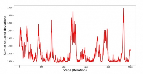
At the very beginning of the descent, we observe a quite uniform and steep reduction in error. In the later iterations, we see that the error fluctuates around the value of 1.475, and at certain moments even reaches this optimal value, but then it still rises again... I reiterate, we could record the coefficient values, and , and then choose those for which the error is minimal. However, we encountered a more serious problem: we had to make 80,000 steps (see the code) to obtain values close to optimal. This contradicts the idea of saving computation time in stochastic gradient descent compared to gradient descent. What can be adjusted and improved? It’s easy to notice that in the first iterations, we confidently move downward, so we should maintain a large step in the early iterations and reduce the step as we progress. We won’t do this in this article — it has already been extended. Interested readers can think about how to do it themselves; it’s not difficult 🙂

Now, let’s perform stochastic gradient descent using the library NumPy (and let’s not stumble over the stones we identified earlier)

Code for stochastic gradient descent (NumPy)

# для начала напишем функцию градиентного шага
def stoch_grad_step_numpy(vector_init, X, ind, y, l):
    x = X[ind]
    y_pred = np.dot(x,vector_init)
    err = y_pred - y[ind]
    grad_a = err
    grad_b = x[1]*err
    return vector_init - l*np.array([grad_a, grad_b])

# определим функцию стохастического градиентного спуска
def stoch_grad_descent_numpy(X, y, l=0.1, steps = 800):
    vector_init = np.array([[np.random.randint(X.shape[0])], [np.random.randint(X.shape[0])]])
    errors = []
    for i in range(steps):
        ind = np.random.randint(X.shape[0])
        new_vector = stoch_grad_step_numpy(vector_init, X, ind, y, l)
        vector_init = new_vector
        errors.append(error_square_numpy(vector_init,X,y))
    return (vector_init), (errors)

# запишем массив значений 
list_parametres_stoch_gradient_descence = stoch_grad_descent_numpy(x_np, y_np, l=0.001, steps = 80000)

print ' 33[1m' + ' 33[4m' + "Значения коэффициентов a и b:" + ' 33[0m'
print 'a =', round(list_parametres_stoch_gradient_descence[0][0],3)
print 'b =', round(list_parametres_stoch_gradient_descence[0][1],3)
print


print ' 33[1m' + ' 33[4m' + "Сумма квадратов отклонений:" + ' 33[0m'
print round(list_parametres_stoch_gradient_descence[1][-1],3)
print



print ' 33[1m' + ' 33[4m' + "Количество итераций в стохастическом градиентном спуске:" + ' 33[0m'
print len(list_parametres_stoch_gradient_descence[1])
print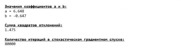

The results were almost the same as when descending without using NumPy. However, this is logical.

Let’s find out how long our stochastic gradient descents took.

Code to determine the computation time of SGD (80,000 steps)

print ' 33[1m' + ' 33[4m' +
"Execution time of stochastic gradient descent without using the NumPy library:"
+ ' 33[0m'
%timeit list_parametres_stoch_gradient_descence = stoch_grad_descent_usual(x_us, y_us, l=0.001, steps = 80000)
print '***************************************'
print

print ' 33[1m' + ' 33[4m' +
"Execution time of stochastic gradient descent using the NumPy library:"
+ ' 33[0m'
%timeit list_parametres_stoch_gradient_descence = stoch_grad_descent_numpy(x_np, y_np, l=0.001, steps = 80000)

The deeper we go into the forest, the darker the clouds: again the 'self-written' formula shows the best result. All this leads to thoughts that there must be even finer ways to utilize the library NumPy, which truly accelerate computational operations. We won't learn about them in this article. It will give us something to think about during our leisure time :)

To summarize

Before summarizing, I would like to address a question that most likely arose for our dear reader. What’s the purpose of these 'torments' with descents? Why go up and down a mountain (mostly down) to find the coveted lowland, when we have such a powerful and simple tool, in the form of an analytical solution, that instantly teleports us to the desired place?

The answer to this question is evident. We have examined a very simple example where the true answer depends on one feature . In reality, this is not often encountered, so let’s imagine we have 2, 30, 50 or more features. On top of that, thousands, or even tens of thousands of values for each feature. In this case, the analytical solution may not withstand the test and fail. In turn, gradient descent and its variations will slowly but surely bring us closer to the target — the function's minimum. And do not worry about the speed — we will definitely explore methods that allow us to set and regulate the step size (i.e., speed).

And now, a brief summary.

First of all, I hope that the material presented in the article helps beginner data scientists understand how to solve simple (and not only) linear regression equations.

Secondly, we have explored several methods for solving the equation. Now, depending on the situation, we can choose the one that best fits our task.

Thirdly, we have seen the power of additional configurations, specifically the step size of gradient descent. This parameter should not be overlooked. As mentioned earlier, to reduce computational costs, the step size should be adjusted during the descent.

Fourthly, in our case, the custom functions demonstrated the best computational time results. This is likely due to not fully utilizing the capabilities of the library. NumPyNevertheless, the conclusion seems clear. On one hand, it is sometimes worth questioning established opinions, and on the other hand, it is not always necessary to complicate matters—sometimes a simpler solution can be more effective. Since our goal was to examine three approaches to solving the equation of simple linear regression, the use of custom functions was sufficient for us.

Literature (or something like that)

1. Linear Regression

http://statistica.ru/theory/osnovy-lineynoy-regressii/

2. Least Squares Method

mathprofi.ru/metod_naimenshih_kvadratov.html

3. Derivative

www.mathprofi.ru/chastnye_proizvodnye_primery.html

4. Gradient

mathprofi.ru/proizvodnaja_po_napravleniju_i_gradient.html

5. Gradient Descent

habr.com/ru/post/471458

habr.com/ru/post/307312

artemarakcheev.com/2017-12-31/linear_regression

6. NumPy Library

docs.scipy.org/doc/numpy-1.10.1/reference/generated/numpy.linalg.solve.html

docs.scipy.org/doc/numpy-1.10.0/reference/generated/numpy.linalg.pinv.html

pythonworld.ru/numpy/2.html

Source: habr.com