

Part Two:
Any raster image can be represented as a two-dimensional matrix. When it comes to colors, the idea can be expanded by considering the image as a three-dimensional matrix, where additional dimensions are used to store data for each of the colors.
If we consider the final color as a combination of so-called primary colors (red, green, and blue), in our three-dimensional matrix we define three planes: the first for red, the second for green, and the last for blue.
We will call each point in this matrix a pixel (element of the image). Each pixel contains information about the intensity (usually in the form of a numerical value) of each color. For example, a red pixel means that it contains 0 green, 0 blue, and maximum red. A pink pixel can be formed using a combination of three colors. Using a numerical range from 0 to 255, a pink pixel is defined as Red = 255, Green = 192 and Blue = 203.
The article is published with the support of EDISON.We develop , and we also specialize in .
Alternative Methods of Encoding Color Images
There are several other models for representing the colors that make up the image. For example, one could use an indexed palette, which requires only one byte to represent each pixel, instead of the three needed when using the RGB model. In such a model, a 2D matrix can be used instead of a 3D matrix to represent each color. This saves memory but offers a smaller color range.
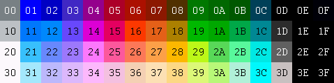
RGB
For example, take a look at the image below. The first face is fully colored. The others are the red, green, and blue planes (the intensity of the respective colors is shown in grayscale).
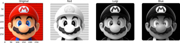
We observe that the shades of red in the original will be in the same places where the brightest parts of the second face are observed. In contrast, the contribution of blue can primarily be seen only in Mario's eyes (the last face) and elements of his clothing. Note where all three color planes contribute the least (the darkest parts of the images) — this is in Mario's mustache.
A certain number of bits is required to store the intensity of each color — this value is called bit depth. Let’s assume 8 bits (ranging from 0 to 255) are spent on one color plane. Then we have a color depth of 24 bits (8 bits * 3 planes R/G/B).
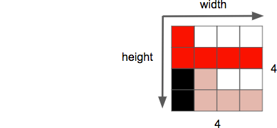
Another property of an image is resolution, which represents the number of pixels in one dimension. It is often denoted as width × height, as demonstrated below in the image example of 4 by 4.
Another property we deal with when working with images/videos is aspect ratio, describing the usual proportional relationship between the width and height of an image or pixel.
When a movie or picture is said to have a size of 16 by 9, it usually refers to the display aspect ratio (DAR — from Display Aspect Ratio). However, there may sometimes be different forms of individual pixels — in this case, we refer to the pixel aspect ratio (PAR — from Pixel Aspect Ratio).
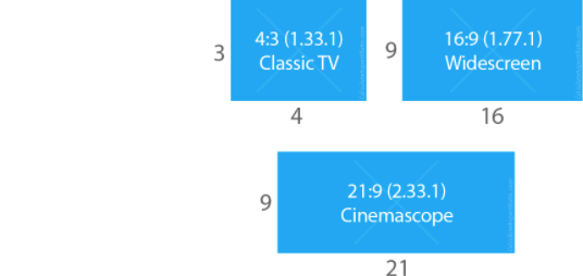
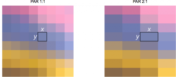
A note for the housekeeper: DVD corresponds to DAR 4 by 3
Although the actual resolution of a DVD is 704×480, it maintains an aspect ratio of 4:3 since the PAR is set at 10:11 (704×10 / 480×11).
Finally, we can define video as a sequence of n frames over a period time, which can be considered an additional dimension. And n then — this is the frame rate or number of frames per second (FPS — from Frames per Second).
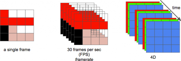
The number of bits per second required to display video is its bitrate — bitrate = width * height * bit depth * frames per second.
For example, for a video with 30 frames per second, 24 bits per pixel, and a resolution of 480×240, it will require 82,944,000 bits per second or 82,944 Mbps (30x480x240x24) — but this is without using any compression methods.
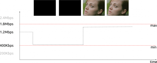
If the bitrate
is almost constant , it is calledconstant bitrate CBR (constant bit rate — from ). But it can also vary; in this case, it is called). But it can also vary; in this case, it's referred to as variable bit rate (VBR — from variable bit rate).
This graph shows limited VBR, where not too many bits are spent in the case of a completely dark frame.
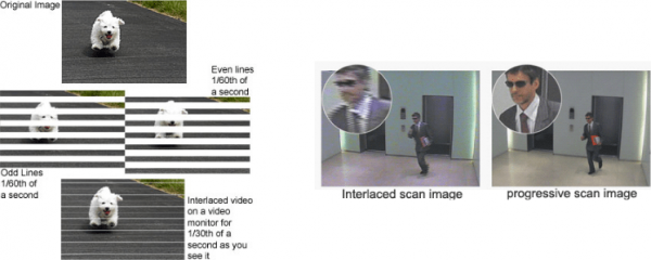
Initially, engineers developed a method to double the perceived frame rate of a display without using additional bandwidth. This method is known as interlaced video; primarily, it sends half of the screen in the first "frame" and the other half in the next "frame."
Currently, scene visualization mainly occurs using progressive scanning technology. This is a method of displaying, storing, or transmitting moving images, where all lines of each frame are drawn sequentially.
Well, now we know how an image is represented digitally, how its colors are arranged, how many bits per second we spend to show video, whether the bit rate is constant (CBR) or variable (VBR). We understand the specified resolution using a given frame rate and are acquainted with many other terms, such as interlaced video, PAR, and some others.
Removing redundancy
It is known that uncompressed video cannot be used effectively. An hour of video at 720p resolution and 30 frames per second would occupy 278 GB. We arrive at this value by multiplying 1280 x 720 x 24 x 30 x 3600 (width, height, bits per pixel, FPS, and time in seconds).
Using lossless compression algorithms, like DEFLATE (used in PKZIP, Gzip, and PNG), will not provide sufficient reduction in required bandwidth. Therefore, we must look for other video compression methods.
To this end, we can leverage the characteristics of our vision. We perceive brightness better than color. Video is a series of sequential images repeated over time. The differences between adjacent frames in the same scene are minor. Furthermore, each frame contains many areas using the same (or similar) color.
Color, brightness, and our eyes
Our eyes are more sensitive to brightness than to color. You can verify this yourself by looking at this image.
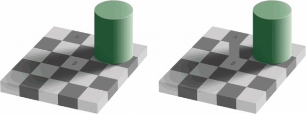
If you cannot see what colors the squares are on the left half of the image. A and B If they are actually the same, that's normal. Our brain causes us to pay more attention to light and shadow rather than color. On the right side between the marked squares, there is a bridge of the same color — hence we (i.e., our brain) can easily determine that, in fact, there is the same color there.
Let's break down (in simplified terms) how our eyes work. The eye is a complex organ made up of many parts. However, we are most interested in the cones and rods. The eye contains about 120 million rods and 6 million cones.
Let's consider color and brightness perception as separate functions of certain parts of the eye (in reality, it's a bit more complex, but we'll simplify). Rod cells primarily respond to brightness, while cone cells respond to color. Cones are divided into three types, depending on the pigment they contain: S-cones (blue), M-cones (green), and L-cones (red).
Since we have significantly more rods (brightness) than cones (color), it can be concluded that we are better at distinguishing transitions between darkness and light than colors.
Contrast Sensitivity Functions
Researchers in experimental psychology and many other fields have developed numerous theories of human vision. One of them is called contrast sensitivity functions. They are related to spatial and temporal illumination. In short, it concerns how many changes are needed before an observer notices them. Note the plural form of the word 'function.' This is because we can measure contrast sensitivity functions not only for black-and-white images but also for color images. Results from these experiments show that in most cases, our eyes are more sensitive to brightness than to color.
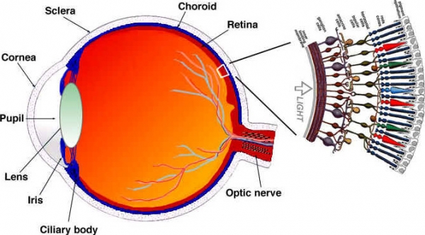
Since it is known that we are more sensitive to the brightness of an image, we can attempt to use this fact.
Color Model
We have somewhat understood how to work with color images using RGB scheme. There are other models as well. There is a model that separates brightness from chroma, known as YCbCr. By the way, there are other models that perform a similar separation, but we will only consider this one.
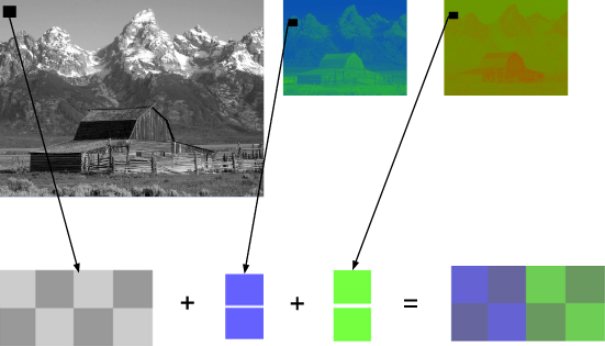
In this color model Y — it represents brightness, and two color channels are used: Cb (saturated blue) and Cr (saturated red). YCbCr can be derived from RGB, and the reverse transformation is also possible. Using this model, we can create full-color images, as shown below:

Conversion between YCbCr and RGB
Someone might argue: how is it possible to obtain all colors without using green?
To answer this question, let’s convert RGB to YCbCr. We will use the coefficients accepted in the standard BT.601, which was recommended by the ITU-R. This division defines standards for digital video. For example: what is 4K? What should be the frame rate, resolution, color model?
First, we will calculate the brightness. We will use the constants proposed by the ITU and substitute the RGB values.
Y = 0.299R + 0.587G + 0.114B
After obtaining the brightness, we will separate the blue and red colors:
Cb = 0.564(B — Y)
Cr = 0.713(R — Y)
And we can also convert back and even obtain green using YCbCr:
R = Y + 1.402Cr
B = Y + 1.772Cb
G = Y — 0.344Cb — 0.714Cr
Generally, displays (monitors, TVs, screens, etc.) use only the RGB model. But this model can be organized in different ways:
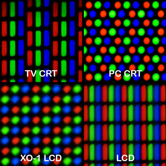
Color Subsampling
With an image represented as a combination of brightness and chrominance, we can take advantage of the human visual system's higher sensitivity to brightness than to chrominance when selectively removing information. Color subsampling is a method of encoding images, using lower resolution for chrominance than for brightness.
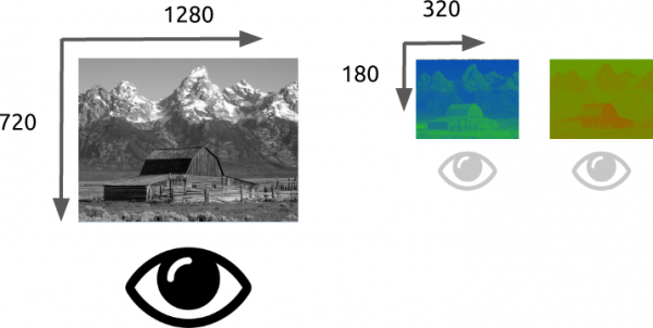
How much can we reduce chrominance resolution?! It turns out there are already some schemes that describe how to handle resolution and merging (Final color = Y + Cb + Cr).
These schemes are known as subsampling systems and are expressed as a 3-to-1 ratio— a:x:y, which defines the number of samples of luminance and chrominance signals.
a — a reference horizontal sampling (usually equal to 4)
x — the number of chrominance samples in the first row of pixels (horizontal resolution relative to a)
y — the number of chrominance sample variations between the first and second rows of pixels.
An exception is 4:1:0, which provides one chrominance sample in every block of luminance resolution 4 by 4.
Common schemes used in modern codecs:
- 4:4:4 (without subsampling)
- 4:2:2
- 4:1:1
- 4:2:0
- 4:1:0
- 3:1:1
YCbCr 4:2:0 — an example of merging
Here is a combined fragment of an image using YCbCr 4:2:0. Note that we only spend 12 bits per pixel.
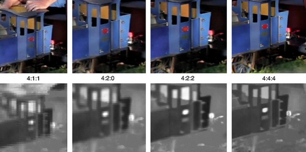
This is how the same image looks encoded with the main types of color subsampling. The top row shows the final YCbCr, while the bottom row displays the chroma resolution. Quite respectable results, considering the minor quality losses.
Remember, we calculated 278 GB of disk space to store an hour of video at 720p resolution and 30 frames per second? If we use YCbCr 4:2:0, that size will be halved to 139 GB. We're still a long way from an acceptable outcome.
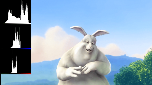
You can create a YCbCr histogram using FFmpeg. In this image, blue prevails over red, which is clearly visible in the histogram itself.
Chroma, brightness, color spectrum — a video overview
I highly recommend watching this amazing video. It explains what brightness is, and essentially clarifies everything about brightness and color.
Types of frames
Let's move on. We'll try to eliminate temporal redundancy. But first, let's define some basic terminology. Let's assume we have a movie with 30 frames per second; here are its first 4 frames:


We can see a lot of repetitions in the frames: for example, the blue background that doesn't change from frame to frame. To address this issue, we can abstractly classify them into three types of frames.
I-frame (IIntro Frame)
An I-frame (intra-frame, keyframe, internal frame) is standalone. Regardless of what needs to be visualized, an I-frame is essentially a static photo. The first frame is usually an I-frame, though we will regularly encounter I-frames among frames that are not first.

P-frame (PPredicted Frame)
A P-frame (predicted frame) takes advantage of the fact that the current image can almost always be constructed using the previous frame. For example, in the second frame, the only change is the ball moving forward. We can get frame 2 simply by slightly modifying frame 1, only using the difference between these frames. To construct frame 2, we refer back to the preceding frame 1.
 ←
← 
B-frame (Bi-predictive Frame)
What about links not only to past frames but also to future ones, to ensure even better compression?! This is essentially what a B-frame (bidirectional frame) is.
 ←
←  →
→ 
Intermediate output
These types of frames are used to achieve the best compression. We will explain how this works in the next section. For now, note that the most 'expensive' in terms of memory used is the I-frame, while the P-frame is significantly cheaper, and the most efficient option for video is the B-frame.

Temporal redundancy (inter-frame prediction)
Let’s consider what options we have to minimize temporal repetitions. This type of redundancy will be resolved through mutual prediction methods.
We will try to use as few bits as possible to encode the sequence of frames 0 and 1.
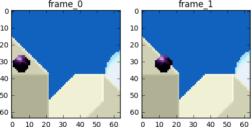
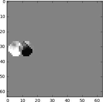
We can perform subtraction, simply subtracting frame 1 from frame 0. We obtain frame 1 using only the difference between it and the previous frame, effectively encoding just the resulting remainder.
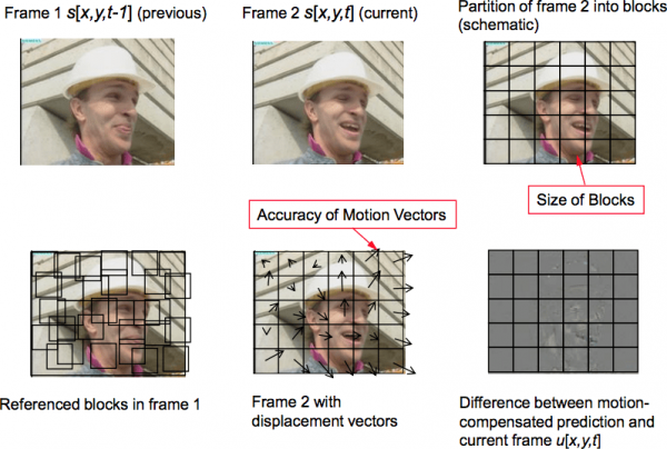
But what if I told you that there’s an even better method that uses even fewer bits?! First, let’s break frame 0 into a clear grid made up of blocks. Then, we will try to match the blocks from frame 0 with those from frame 1. In other words, we will assess the motion between frames.
From Wikipedia — block motion compensation
Block motion compensation divides the current frame into non-overlapping blocks, and the motion compensation vector indicates the origin of the blocks (a common misconception is that the previous frame is divided into non-overlapping blocks, and the motion compensation vectors indicate where those blocks are moving. In fact, it’s the other way around — the analysis is done not on the previous frame but on the subsequent one, determining not where the blocks move, but where they originated from). Typically, the original blocks overlap in the source frame. Some video compression algorithms reconstruct the current frame from parts of not just one but several previously transmitted frames.
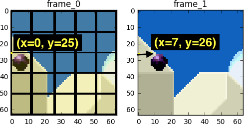
During the evaluation, we see that the ball has moved from (x=0, y=25) to (x=6, y=26), values x and y define the motion vector. Another step we can take to preserve bits is to encode only the difference in motion vectors between the block's last position and the predicted one, so the final motion vector will be (x=6-0=6, y=26-25=1).
In a real scenario, this ball would be divided into n blocks, but that doesn't change the essence of the matter.
Objects in the frame move in three dimensions, so when the ball moves, it may appear visually smaller (or larger if moving towards the viewer). It's normal that there won't be a perfect match between the blocks. Here is a combined view of our estimation and the real picture.
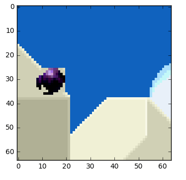
But we see that when we apply motion estimation, the data for encoding is noticeably less than when using the simpler method of calculating the delta between frames.
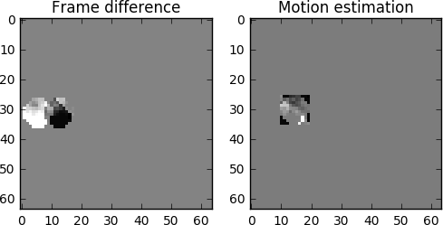
What real motion compensation will look like
This technique is applied to all blocks at once. Often our hypothetical moving ball will be split into several blocks.
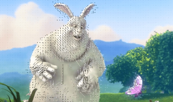
You can experiment with these concepts by using .
To visualize motion vectors, you can create a video with external prediction using .
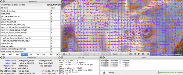
You can also use (it's paid, but there is a free trial version limited to just the first ten frames).
Spatial redundancy (internal prediction)
If we analyze each frame in the video, we will find many interrelated areas.
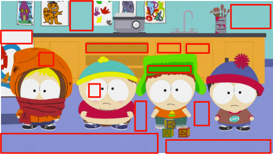
Let's walk through this example. This scene mainly consists of blue and white colors.

This is an I-frame. We cannot use previous frames for prediction, but we can compress it. We will encode the red block's selection. If we look at its neighbors, we notice that there are some color trends around it.
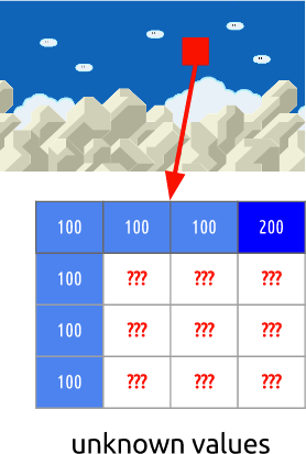
We assume that colors in the frame spread vertically. This means that the color values of unknown pixels will be influenced by the values of their neighbors.
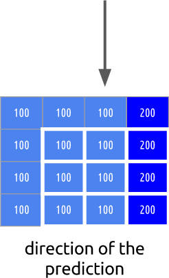
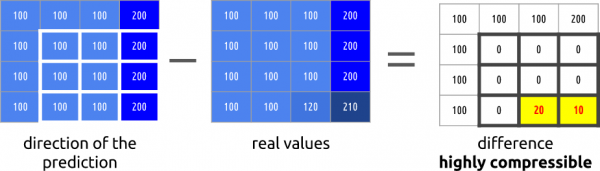
Such a prediction may also be incorrect. For this reason, we need to apply this method (internal prediction) and then subtract the actual values. This will give us a residual block, leading to a much more compact matrix compared to the original.
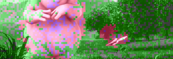
If you want to practice with internal predictions, you can create a video with macro blocks and their predictions using ffmpeg. To understand the meaning of each block color, you'll need to refer to the ffmpeg documentation.
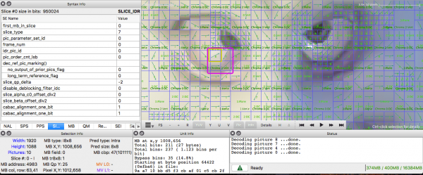
Alternatively, you can use Intel Video Pro Analyzer (as I mentioned earlier, the trial version is limited to the first 10 frames, but that should be sufficient for your initial needs).
Part Two:
Source: habr.com
