🥇Your First Neural Network on a Graphics Processor (GPU). A Beginner's Guide

In this article, I will explain how to set up a machine learning environment in 30 minutes, create a neural network for image recognition, and then run the same network on a Graphics Processing Unit (GPU).

First, let's define what a neural network is.

In our case, it is a mathematical model, as well as its software or hardware implementation, built on the principles of organization and functioning of biological neural networks—the networks of nerve cells of living organisms. This concept arose from the study of processes occurring in the brain and attempts to model these processes.

Neural networks are not programmed in the traditional sense of the word; they are trained. The ability to learn is one of the main advantages of neural networks over traditional algorithms. Technically, learning consists of finding the coefficients of connections between neurons. During the training process, a neural network is capable of identifying complex relationships between input and output data, as well as performing generalization.

From the perspective of machine learning, a neural network is a specific case of pattern recognition methods, discriminant analysis, clustering methods, and other methods.

Hardware

First, let's discuss the hardware. We need a server with a Linux operating system installed on it. The hardware required for machine learning systems needs to be quite powerful and, consequently, expensive. For those who do not have a good machine at hand, I recommend looking at the offers from cloud providers. The necessary server can be rented quickly, and you only pay for the time you use.

In projects that require the creation of neural networks, I use servers from one of the Russian cloud providers. The company offers rental cloud servers specifically for machine learning with powerful Tesla V100 graphics processing units (GPUs) from NVIDIA. In short, using a server with a GPU can be tens of times more effective (faster) compared to a similarly priced server where computing is done using a CPU (the well-known central processor). This is achieved due to the architecture of the GPU, which handles calculations more swiftly.

To run the examples described below, we rented such a server for a few days:

150 GB SSD
32 GB RAM
Tesla V100 16 GB processor with 4 cores

They installed Ubuntu 18.04 on our machine.

Setting up the environment

Now let's install everything necessary for the server to function. Since this article is primarily targeted at beginners, I will discuss some aspects that will be particularly useful to them.

A lot of work in setting up the environment is done through the command line. Most users use Windows as their operating system. The standard console in this OS leaves much to be desired. Therefore, we will use a convenient tool Cmder/. We download the mini version and launch Cmder.exe. Next, we need to connect to the server via SSH protocol:

ssh root@server-ip-or-hostname

Replace server-ip-or-hostname with your server's IP address or DNS name. Then enter the password, and upon successful connection, you should see a message like this.

Welcome to Ubuntu 18.04.3 LTS (GNU/Linux 4.15.0-74-generic x86_64)

The main programming language for developing ML models is Python. The most popular platform for using it on Linux is Anaconda.

Let's install it on our server.

We start by updating the local package manager:

sudo apt-get update

Installing curl (a command-line utility):

sudo apt-get install curl

Download the latest version of Anaconda Distribution:

cd /tmp
curl –O https://repo.anaconda.com/archive/Anaconda3-2019.10-Linux-x86_64.sh

Start the installation:

bash Anaconda3-2019.10-Linux-x86_64.sh

During the installation process, you will have to accept the license agreement. Upon successful installation, you should see this:

Thank you for installing Anaconda3!

There are many frameworks created for ML model development now, and we work with the most popular ones: PyTorch and Tensorflow.

Using a framework allows for faster development and the utilization of ready-made tools for standard tasks.

In this example, we will work with PyTorch. Let's install it:

conda install pytorch torchvision cudatoolkit=10.1 -c pytorch

Now we need to launch Jupyter Notebook — a popular development tool among ML specialists. It allows you to write code and immediately see the results of its execution. Jupyter Notebook is part of Anaconda and is already installed on our server. We need to connect to it from our desktop system.

To do this, we first start Jupyter on the server specifying port 8080:

jupyter notebook --no-browser --port=8080 --allow-root

Next, by opening another tab in our Cmder console (top menu — New console dialog), we will connect via SSH to the server through port 8080:

ssh -L 8080:localhost:8080 root@server-ip-or-hostname

When entering the first command, we will be provided with links to open Jupyter in our browser:

To access the notebook, open this file in a browser:
        file:///root/.local/share/jupyter/runtime/nbserver-18788-open.html
    Or copy and paste one of these URLs:
        http://localhost:8080/?token=cca0bd0b30857821194b9018a5394a4ed2322236f116d311
     or http://127.0.0.1:8080/?token=cca0bd0b30857821194b9018a5394a4ed2322236f116d311

We will use the link for localhost:8080. Copy the full path and paste it into the address bar of your local browser. Jupyter Notebook will open.

Let's create a new notebook: New — Notebook — Python 3.

We will check the correct operation of all the components we installed. Enter the PyTorch example code in Jupyter and run it (click the Run button):

from __future__ import print_function
import torch
x = torch.rand(5, 3)
print(x)

The result should look something like this:

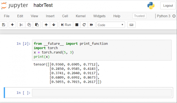
If you have a similar result, it means we have configured everything correctly and can proceed to develop the neural network!

Creating a Neural Network

We will create a neural network for image recognition. We will take as a basis guide.

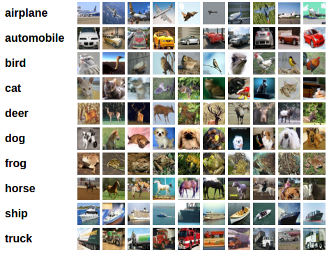
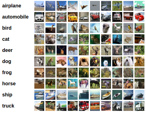
For training the network, we will use the publicly available CIFAR10 dataset. It has classes: 'airplane', 'car', 'bird', 'cat', 'deer', 'dog', 'frog', 'horse', 'ship', 'truck'. Images in CIFAR10 are 3x32x32, meaning 3-channel color images sized 32×32 pixels.

For our work, we will use the created PyTorch package for image processing — torchvision.

We will follow these steps in order:

Loading and normalizing training and test datasets
Defining the neural network
Training the network on the training data
Testing the network on the test data
We will repeat training and testing using the GPU

All the code below will be executed in Jupyter Notebook.

Loading and normalizing CIFAR10

Copy and execute the following code in Jupyter:


import torch
import torchvision
import torchvision.transforms as transforms

transform = transforms.Compose(
    [transforms.ToTensor(),
     transforms.Normalize((0.5, 0.5, 0.5), (0.5, 0.5, 0.5))])

trainset = torchvision.datasets.CIFAR10(root='./data', train=True,
                                        download=True, transform=transform)
trainloader = torch.utils.data.DataLoader(trainset, batch_size=4,
                                          shuffle=True, num_workers=2)

testset = torchvision.datasets.CIFAR10(root='./data', train=False,
                                       download=True, transform=transform)
testloader = torch.utils.data.DataLoader(testset, batch_size=4,
                                         shuffle=False, num_workers=2)

classes = ('plane', 'car', 'bird', 'cat',
           'deer', 'dog', 'frog', 'horse', 'ship', 'truck')

The output should be as follows:

Downloading https://www.cs.toronto.edu/~kriz/cifar-10-python.tar.gz to ./data/cifar-10-python.tar.gz
Extracting ./data/cifar-10-python.tar.gz to ./data
Files already downloaded and verified

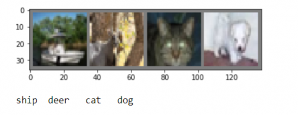
Let's display a few training samples for verification:


import matplotlib.pyplot as plt
import numpy as np

# functions to show an image

def imshow(img):
    img = img / 2 + 0.5     # unnormalize
    npimg = img.numpy()
    plt.imshow(np.transpose(npimg, (1, 2, 0)))
    plt.show()

# get some random training images
dataiter = iter(trainloader)
images, labels = dataiter.next()

# show images
imshow(torchvision.utils.make_grid(images))
# print labels
print(' '.join('%5s' % classes[labels[j]] for j in range(4)))

Defining the neural network

First, let's understand how the image recognition neural network works. This is a simple feedforward network. It takes input data, passes it through several layers one by one, and finally outputs results.

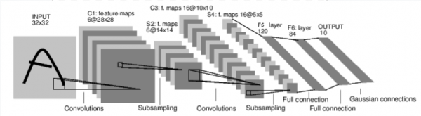
Let's create a similar network in our environment:


import torch.nn as nn
import torch.nn.functional as F

class Net(nn.Module):
    def __init__(self):
        super(Net, self).__init__()
        self.conv1 = nn.Conv2d(3, 6, 5)
        self.pool = nn.MaxPool2d(2, 2)
        self.conv2 = nn.Conv2d(6, 16, 5)
        self.fc1 = nn.Linear(16 * 5 * 5, 120)
        self.fc2 = nn.Linear(120, 84)
        self.fc3 = nn.Linear(84, 10)

    def forward(self, x):
        x = self.pool(F.relu(self.conv1(x)))
        x = self.pool(F.relu(self.conv2(x)))
        x = x.view(-1, 16 * 5 * 5)
        x = F.relu(self.fc1(x))
        x = F.relu(self.fc2(x))
        x = self.fc3(x)
        return x

net = Net()

We will also define the loss function and the optimizer


import torch.optim as optim

criterion = nn.CrossEntropyLoss()
optimizer = optim.SGD(net.parameters(), lr=0.001, momentum=0.9)

Training the network on the training data

We are starting the training of our neural network. Please note that after you run this code, you will need to wait a while for it to finish. It took me about 5 minutes. Training the network requires time.

 for epoch in range(2): # loop over the dataset multiple times

 running_loss = 0.0
 for i, data in enumerate(trainloader, 0):
 # get the inputs; data is a list of [inputs, labels]
 inputs, labels = data

 # zero the parameter gradients
 optimizer.zero_grad()

 # forward + backward + optimize
 outputs = net(inputs)
 loss = criterion(outputs, labels)
 loss.backward()
 optimizer.step()

 # print statistics
 running_loss += loss.item()
 if i % 2000 == 1999: # print every 2000 mini-batches
 print('[%d, ] loss: %.3f' %
 (epoch + 1, i + 1, running_loss / 2000))
 running_loss = 0.0

print('Finished Training')

We will get a result like this:

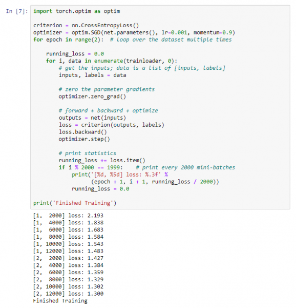
Saving our trained model:

PATH = './cifar_net.pth'
torch.save(net.state_dict(), PATH)

Testing the network on the test data

We have trained the network using a training dataset. But we need to check if the network has actually learned anything.

We will verify this by predicting the class label that the neural network outputs and checking it for accuracy. If the prediction is correct, we will add the sample to the list of correct predictions.
Let's show an image from the test set:

dataiter = iter(testloader)
images, labels = dataiter.next()

# print images
imshow(torchvision.utils.make_grid(images))
print('GroundTruth: ', ' '.join('%5s' % classes[labels[j]] for j in range(4)))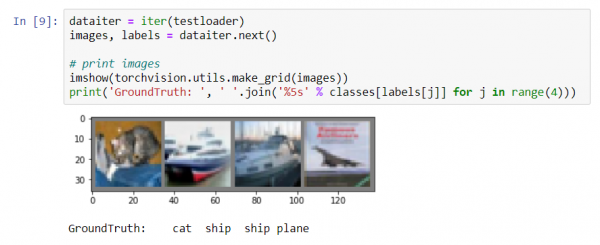

Now let's ask the neural network to tell us what is in these images:


net = Net()
net.load_state_dict(torch.load(PATH))

outputs = net(images)

_, predicted = torch.max(outputs, 1)

print('Predicted: ', ' '.join('%5s' % classes[predicted[j]]
                              for j in range(4)))

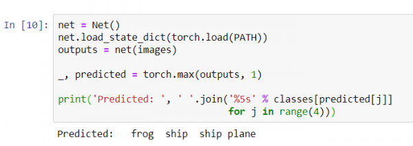
The results seem quite good: the network correctly identified three out of four images.

Let's see how the network performs across the entire dataset.


correct = 0
total = 0
with torch.no_grad():
    for data in testloader:
        images, labels = data
        outputs = net(images)
        _, predicted = torch.max(outputs.data, 1)
        total += labels.size(0)
        correct += (predicted == labels).sum().item()

print('Accuracy of the network on the 10000 test images: %d %%' % (
    100 * correct / total))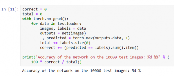

It seems the network knows something and is working. If it were guessing classes randomly, the accuracy would be 10%.

Now let's see which classes the network identifies better:

class_correct = list(0. for i in range(10))
class_total = list(0. for i in range(10))
with torch.no_grad():
 for data in testloader:
 images, labels = data
 outputs = net(images)
 _, predicted = torch.max(outputs, 1)
 c = (predicted == labels).squeeze()
 for i in range(4):
 label = labels[i]
 class_correct[label] += c[i].item()
 class_total[label] += 1


for i in range(10):
 print('Accuracy of %5s : %%' % (
 classes[i], 100 * class_correct[i] / class_total[i]))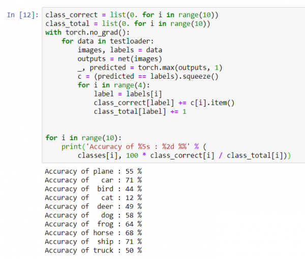

It seems that the network performs best in identifying cars and ships: 71% accuracy.

So the network is working. Now let's try to transfer its operation to the graphics processor (GPU) and see what changes.

Training the neural network on the GPU

First, let me briefly explain what CUDA is. CUDA (Compute Unified Device Architecture) is a parallel computing platform developed by NVIDIA for general-purpose computations on graphics processors (GPUs). Using CUDA, developers can significantly accelerate computational applications by leveraging the capabilities of graphics processors. The platform is already installed on our server that we purchased.

First, let's define our GPU as the first visible CUDA device.

device = torch.device("cuda:0" if torch.cuda.is_available() else "cpu")
# Assuming that we are on a CUDA machine, this should print a CUDA device:
print(device)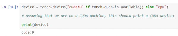

Sending the network to the GPU:

net.to(device)

We will also have to send inputs and targets at each step to the GPU:

inputs, labels = data[0].to(device), data[1].to(device)

Let's run the retraining of the network already on the GPU:

import torch.optim as optim

criterion = nn.CrossEntropyLoss()
optimizer = optim.SGD(net.parameters(), lr=0.001, momentum=0.9)
for epoch in range(2): # loop over the dataset multiple times

 running_loss = 0.0
 for i, data in enumerate(trainloader, 0):
 # get the inputs; data is a list of [inputs, labels]
 inputs, labels = data[0].to(device), data[1].to(device)

 # zero the parameter gradients
 optimizer.zero_grad()

 # forward + backward + optimize
 outputs = net(inputs)
 loss = criterion(outputs, labels)
 loss.backward()
 optimizer.step()

 # print statistics
 running_loss += loss.item()
 if i % 2000 == 1999: # print every 2000 mini-batches
 print('[%d, ] loss: %.3f' %
 (epoch + 1, i + 1, running_loss / 2000))
 running_loss = 0.0

print('Finished Training')

This time, the training of the network lasted about 3 minutes. Remember that the same stage on a regular processor took 5 minutes. The difference isn't significant; this is because our network isn't that large. When using larger datasets for training, the speed difference between the GPU and traditional processor will increase.

That seems to be all. Here’s what we were able to achieve: