

This note will be of interest to those using the data processing library for R — data.table, and may appreciate the flexibility of its application across various examples.
Inspired by a good example , and hoping you have already read its article, I suggest delving deeper into code optimization and performance based on data.table.
Introduction: Where does data.table come from?
The best way to start getting acquainted with the library is to begin from afar, specifically with the data structures from which a data.table (hereinafter, DT) object can be derived.
Array
Code
## arrays ---------

arrmatr <- array(1:20, c(4,5))

class(arrmatr)

typeof(arrmatr)

is.array(arrmatr)

is.matrix(arrmatr)
One such structure is an array (?base::array). Like in other languages, arrays here are multidimensional. However, it is interesting that, for example, a two-dimensional array starts inheriting properties from the matrix class (?base::matrix), while a one-dimensional array, which is also important, does not inherit from a vector (?base::vector).
It should be understood that the data type contained in any object should be checked using the function base::typeof, which returns the internal description of the type according to R Internals — the general protocol of the language related to the primordial C.
Another command for determining the class of an object, base::class, returns a vector type in the case of vectors (it has a different name from the internal type, but also allows understanding the data type).
List
From a two-dimensional array, i.e., a matrix, one can transition to a list (?base::list).
Code
## lists ------------------

mylist <- as.list(arrmatr)

is.vector(mylist)

is.list(mylist)
Several things happen at once:
- The second dimension of the matrix collapses, meaning we obtain both a list and a vector at once.
- Thus, a list inherits from these classes. It should be noted that a list element will correspond to one (scalar) value from the matrix-array cell.
Due to the fact that a list is also a vector, some functions for vectors can be applied to it.
Data frame
From a list, a matrix, or a vector, one can transition to a data frame (?base::data.frame).
Code
## data.frames ------------

df <- as.data.frame(arrmatr)
df2 <- as.data.frame(mylist)

is.list(df)

df$V6 <- df$V1 + df$V2
What's interesting about it: a data frame inherits from a list! The columns of the data frame are the cells of the list. This will be important later when we use functions applicable to lists.
data.table
You can obtain a DT (?data.table::data.table) from a data frame, a list, a vector, or a matrix. For example, like this (in place).
Code
## data.tables -----------------------
library(data.table)

data.table::setDT(df)

is.list(df)

is.data.frame(df)

is.data.table(df)
What’s useful is that, like a data frame, DT inherits properties from a list.
DT and memory
Unlike all other objects in R base, DTs are passed by reference. If you need to make a copy in a new memory area, you need the function data.table::copy or you need to make a selection from the old object.
Code
df2 <- df

df[V1 == 1, V2 := 999]

data.table::fsetdiff(df, df2)

df2 <- data.table::copy(df)

df[V1 == 2, V2 := 999]

data.table::fsetdiff(df, df2)
This introduction is coming to an end. DT is a continuation of the development of data structures in R, which primarily happens through the expansion and acceleration of operations performed on objects of class data frame. In this process, inheritance from other primitives is maintained.
Some examples of using data.table properties
Like a list…
Iterating over the rows of a data frame or DT is not the best idea, as the loop code in the language R is significantly slower C, while iterating over columns, which are usually significantly fewer in number, is quite feasible. When going through columns, remember that each column is an element of a list, typically containing a vector. Vector operations are well vectorized in the basic functions of the language. You can also use selection operators characteristic of lists and vectors: `[[`, `$`.
Code
## operations on data.tables ------------

#using list properties

df$'V1'[1]

df[['V1']]

df[[1]][1]

sapply(df, class)

sapply(df, function(x) sum(is.na(x)))
Vectorization
If there is a need to iterate over the rows of a large DT, the best solution would be to write a function with vectorization. However, if that’s not possible, keep in mind that the DT loop is still faster than the loop in inside , as it runs on RLet's try on a larger example with 100K rows. We will extract the first letter from the words contained in a vector-column. C.
Updated w.
library(magrittr) library(microbenchmark)## Bigger example ----rown <- 100000dt % .[, d := 1 + b + c + rnorm(nrow(.))]# vectorizationmicrobenchmark({ dt[ , first_l := unlist(strsplit(w, split = ' ', fixed = T))[1] , by = 1:nrow(dt) ] })# secondfirst_l_f % do.call(rbind, .) %>% `[`(,1) }dt[, first_l := NULL]microbenchmark({ dt[ , first_l := .(first_l_f(w)) ] })# thirdfirst_l_f2 % unlist %>% matrix(nrow = 3) %>% `[`(1,) }dt[, first_l := NULL]microbenchmark({ dt[ , first_l := .(first_l_f2(w)) ] })
Code
First run with iteration over rows:
Unit: milliseconds
expr min
{ dt[, `:=`(first_l, unlist(strsplit(w, split = " ", fixed = T))[1]), by = 1:nrow(dt)] } 439.6217
lq mean median uq max neval
lq mean median uq max neval
451.9998 460.1593 456.2505 460.9147 621.4042 100
The second run, where vectorization occurs through converting a list into a matrix and taking elements from the slice with index 1 (which is essentially the vectorization itself). I will correct myself: vectorization at the function level. strsplit, which can accept a vector as input. It turns out that the procedure for converting a list into a matrix is much heavier than the vectorization itself, but even in this case, it is significantly faster than the non-vectorized option.
expr min
expr min lq mean median uq max neval
{ dt[, `:=`(first_l, .(first_l_f(w)))] } 93.07916 112.1381 161.9267 149.6863 185.9893 442.5199 100
Speedup by median in 3 times.
The third run, where the scheme for converting to a matrix has been changed.
expr min
expr min lq mean median uq max neval
{ dt[, `:=`(first_l, .(first_l_f2(w)))] } 32.60481 34.13679 40.4544 35.57115 42.11975 222.972 100
Speedup by median in 13 times.
One needs to experiment with this; the more, the better it will be.
Another example with vectorization, where the text is also involved, but it is closer to real conditions: different word lengths, different numbers of words. The goal is to extract the first 3 words. Like this:
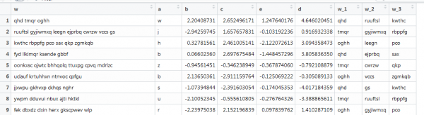
Here, the previous function does not work already, as the vectors are of different lengths, and we set the size of the matrix. We will redo this by searching the internet.
Code
# fourth

rown <- 100000

words <-
	sapply(
		seq_len(rown)
		, function(x){
			nwords <- rbinom(1, 10, 0.5)
			paste(
				sapply(
					seq_len(nwords)
					, function(x){
						paste(sample(letters, rbinom(1, 10, 0.5), replace = T), collapse = '')
					}
				)
				, collapse = ' '
			)
		}
	)

dt <-
	data.table(
		w = words
		, a = sample(letters, rown, replace = T)
		, b = runif(rown, -3, 3)
		, c = runif(rown, -3, 3)
		, e = rnorm(rown)
	) %>%
	.[, d := 1 + b + c + rnorm(nrow(.))]

first_l_f3 <- function(sd, n)
{
	l <- strsplit(sd, split = ' ', fixed = T)

	maxl <- max(lengths(l))

	sapply(l, "length<-", maxl) %>%
		`[`(n,) %>%
		as.character
}

microbenchmark({
	dt[
		, (paste0('w_', 1:3)) := lapply(1:3, function(x) first_l_f3(w, x))
		]
})

dt[
	, (paste0('w_', 1:3)) := lapply(1:3, function(x) first_l_f3(w, x))
	]
expr min
expr min lq mean median
{ dt[, `:=`((paste0("w_", 1:3)), strsplit(w, split = " ", fixed = T))] } 851.7623 916.071 1054.5 1035.199
uq max neval
1178.738 1356.816 100
The script ran with an average speed of 1 second. Not bad.
Connected in a chain…
You can work with DT objects using chaining. It looks like appending bracket syntax to the right, essentially a sweetener.
Code
# chaining

res1 <- dt[a == 'a'][sample(.N, 100)]

res2 <- dt[, .N, a][, N]

res3 <- dt[, coefficients(lm(e ~ d))[1], a][, .(letter = a, coef = V1)]
Flowing through the pipes…
Similar operations can be done through piping; it looks similar but is functionally richer, as you can use any methods, not just DT. We will output the coefficients of logistic regression for our synthetic data with a series of filters on DT.
Code
# piping

samplpe_b <- dt[a %in% head(letters), sample(b, 1)]

res4 <-
	dt %>%
	.[a %in% head(letters)] %>%
	.[,
	  {
	  	dt0 <- .SD[1:100]

	  	quants <-
	  		dt0[, c] %>%
	  		quantile(seq(0.1, 1, 0.1), na.rm = T)

	  	.(q = quants)
	  }
	  , .(cond = b > samplpe_b)
	  ] %>%
	glm(
		cond ~ q -1
		, family = binomial(link = "logit")
		, data = .
	) %>%
	summary %>%
	.[[12]]
Statistics, machine learning, and more within DT
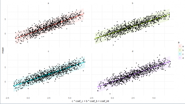
You can use lambda functions, but sometimes it's better to create them separately, write out the entire data analysis pipeline, and proceed — they work within DT. The example is enriched with all the aforementioned features, plus a few useful things from the DT arsenal (such as referring to DT itself within DT via a link, inserted sometimes non-sequentially, but just to have it).
Code
# function

rm(lm_preds)

lm_preds <- function(
	sd, by, n
)
{

	if(
		n < 100 |
		!by[['a']] %in% head(letters, 4)
	   )
	{

		res <-
			list(
				low = NA
				, mean = NA
				, high = NA
				, coefs = NA
			)

	} else {

		lmm <-
			lm(
				d ~ c + b
				, data = sd
			)

		preds <-
			stats::predict.lm(
				lmm
				, sd
				, interval = "prediction"
				)

		res <-
			list(
				low = preds[, 2]
				, mean = preds[, 1]
				, high = preds[, 3]
				, coefs = coefficients(lmm)
			)
	}

	res

}

res5 <-
	dt %>%
	.[e < 0] %>%
	.[.[, .I[b > 0]]] %>%
	.[, `:=` (
		low = as.numeric(lm_preds(.SD, .BY, .N)[[1]])
		, mean = as.numeric(lm_preds(.SD, .BY, .N)[[2]])
		, high = as.numeric(lm_preds(.SD, .BY, .N)[[3]])
		, coef_c = as.numeric(lm_preds(.SD, .BY, .N)[[4]][1])
		, coef_b = as.numeric(lm_preds(.SD, .BY, .N)[[4]][2])
		, coef_int = as.numeric(lm_preds(.SD, .BY, .N)[[4]][3])
	)
	, a
	] %>%
	.[!is.na(mean), -'e', with = F]


# plot

plo <-
	res5 %>%
	ggplot +
	facet_wrap(~ a) +
	geom_ribbon(
		aes(
			x = c * coef_c + b * coef_b + coef_int
			, ymin = low
			, ymax = high
			, fill = a
		)
		, size = 0.1
		, alpha = 0.1
	) +
	geom_point(
		aes(
			x = c * coef_c + b * coef_b + coef_int
			, y = mean
			, color = a
		)
		, size = 1
	) +
	geom_point(
		aes(
			x = c * coef_c + b * coef_b + coef_int
			, y = d
		)
		, size = 1
		, color = 'black'
	) +
	theme_minimal()

print(plo)
Conclusion
I hope I was able to create a coherent, though certainly not complete, picture of an object like data.table, starting from its properties related to R class inheritance and ending with its own features and the environment of tidyverse elements. I hope this helps you better learn and apply this library for work and entertainment.
Thank you!
Full Code
Code
## load libs ----------------

library(data.table)
library(ggplot2)
library(magrittr)
library(microbenchmark)


## arrays ---------

arrmatr <- array(1:20, c(4,5))

class(arrmatr)

typeof(arrmatr)

is.array(arrmatr)

is.matrix(arrmatr)


## lists ------------------

mylist <- as.list(arrmatr)

is.vector(mylist)

is.list(mylist)


## data.frames ------------

df <- as.data.frame(arrmatr)

is.list(df)

df$V6 <- df$V1 + df$V2


## data.tables -----------------------

data.table::setDT(df)

is.list(df)

is.data.frame(df)

is.data.table(df)

df2 <- df

df[V1 == 1, V2 := 999]

data.table::fsetdiff(df, df2)

df2 <- data.table::copy(df)

df[V1 == 2, V2 := 999]

data.table::fsetdiff(df, df2)


## operations on data.tables ------------

#using list properties

df$'V1'[1]

df[['V1']]

df[[1]][1]

sapply(df, class)

sapply(df, function(x) sum(is.na(x)))


## Bigger example ----

rown <- 100000

dt <-
	data.table(
		w = sapply(seq_len(rown), function(x) paste(sample(letters, 3, replace = T), collapse = ' '))
		, a = sample(letters, rown, replace = T)
		, b = runif(rown, -3, 3)
		, c = runif(rown, -3, 3)
		, e = rnorm(rown)
	) %>%
	.[, d := 1 + b + c + rnorm(nrow(.))]

# vectorization

# zero - for loop

microbenchmark({
	for(i in 1:nrow(dt))
		{
		dt[
			i
			, first_l := unlist(strsplit(w, split = ' ', fixed = T))[1]
		]
	}
})

# first

microbenchmark({
	dt[
		, first_l := unlist(strsplit(w, split = ' ', fixed = T))[1]
		, by = 1:nrow(dt)
	   ]
})

# second

first_l_f <- function(sd)
{
	strsplit(sd, split = ' ', fixed = T) %>%
		do.call(rbind, .) %>%
		`[`(,1)
}

dt[, first_l := NULL]

microbenchmark({
	dt[
		, first_l := .(first_l_f(w))
		]
})

# third

first_l_f2 <- function(sd)
{
	strsplit(sd, split = ' ', fixed = T) %>%
		unlist %>%
		matrix(nrow = 3) %>%
		`[`(1,)
}

dt[, first_l := NULL]

microbenchmark({
	dt[
		, first_l := .(first_l_f2(w))
		]
})

# fourth

rown <- 100000

words <-
	sapply(
		seq_len(rown)
		, function(x){
			nwords <- rbinom(1, 10, 0.5)
			paste(
				sapply(
					seq_len(nwords)
					, function(x){
						paste(sample(letters, rbinom(1, 10, 0.5), replace = T), collapse = '')
					}
				)
				, collapse = ' '
			)
		}
	)

dt <-
	data.table(
		w = words
		, a = sample(letters, rown, replace = T)
		, b = runif(rown, -3, 3)
		, c = runif(rown, -3, 3)
		, e = rnorm(rown)
	) %>%
	.[, d := 1 + b + c + rnorm(nrow(.))]

first_l_f3 <- function(sd, n)
{
	l <- strsplit(sd, split = ' ', fixed = T)

	maxl <- max(lengths(l))

	sapply(l, "length<-", maxl) %>%
		`[`(n,) %>%
		as.character
}

microbenchmark({
	dt[
		, (paste0('w_', 1:3)) := lapply(1:3, function(x) first_l_f3(w, x))
		]
})

dt[
	, (paste0('w_', 1:3)) := lapply(1:3, function(x) first_l_f3(w, x))
	]


# chaining

res1 <- dt[a == 'a'][sample(.N, 100)]

res2 <- dt[, .N, a][, N]

res3 <- dt[, coefficients(lm(e ~ d))[1], a][, .(letter = a, coef = V1)]

# piping

samplpe_b <- dt[a %in% head(letters), sample(b, 1)]

res4 <-
	dt %>%
	.[a %in% head(letters)] %>%
	.[,
	  {
	  	dt0 <- .SD[1:100]

	  	quants <-
	  		dt0[, c] %>%
	  		quantile(seq(0.1, 1, 0.1), na.rm = T)

	  	.(q = quants)
	  }
	  , .(cond = b > samplpe_b)
	  ] %>%
	glm(
		cond ~ q -1
		, family = binomial(link = "logit")
		, data = .
	) %>%
	summary %>%
	.[[12]]


# function

rm(lm_preds)

lm_preds <- function(
	sd, by, n
)
{

	if(
		n < 100 |
		!by[['a']] %in% head(letters, 4)
	   )
	{

		res <-
			list(
				low = NA
				, mean = NA
				, high = NA
				, coefs = NA
			)

	} else {

		lmm <-
			lm(
				d ~ c + b
				, data = sd
			)

		preds <-
			stats::predict.lm(
				lmm
				, sd
				, interval = "prediction"
				)

		res <-
			list(
				low = preds[, 2]
				, mean = preds[, 1]
				, high = preds[, 3]
				, coefs = coefficients(lmm)
			)
	}

	res

}

res5 <-
	dt %>%
	.[e < 0] %>%
	.[.[, .I[b > 0]]] %>%
	.[, `:=` (
		low = as.numeric(lm_preds(.SD, .BY, .N)[[1]])
		, mean = as.numeric(lm_preds(.SD, .BY, .N)[[2]])
		, high = as.numeric(lm_preds(.SD, .BY, .N)[[3]])
		, coef_c = as.numeric(lm_preds(.SD, .BY, .N)[[4]][1])
		, coef_b = as.numeric(lm_preds(.SD, .BY, .N)[[4]][2])
		, coef_int = as.numeric(lm_preds(.SD, .BY, .N)[[4]][3])
	)
	, a
	] %>%
	.[!is.na(mean), -'e', with = F]


# plot

plo <-
	res5 %>%
	ggplot +
	facet_wrap(~ a) +
	geom_ribbon(
		aes(
			x = c * coef_c + b * coef_b + coef_int
			, ymin = low
			, ymax = high
			, fill = a
		)
		, size = 0.1
		, alpha = 0.1
	) +
	geom_point(
		aes(
			x = c * coef_c + b * coef_b + coef_int
			, y = mean
			, color = a
		)
		, size = 1
	) +
	geom_point(
		aes(
			x = c * coef_c + b * coef_b + coef_int
			, y = d
		)
		, size = 1
		, color = 'black'
	) +
	theme_minimal()

print(plo)
Source: habr.com
