🥇What EXPLAIN is silent about, and how to get it talking

A classic question that every developer asks their DBA or business owner to a PostgreSQL consultant almost always sounds the same: "Why are the queries taking so long to execute on the database?"

A traditional set of reasons:

inefficient algorithm
when you decide to JOIN several CTEs with a couple of tens of thousands of records
outdated statistics
if the actual distribution of data in the table has significantly changed since the last ANALYZE
"bottleneck" in resources
and there are no longer enough allocated CPU computing resources, with gigabytes of memory constantly being processed or the disk can't keep up with all the database "wants"
locks from competing processes

And if locks are complicated enough to capture and analyze, for everything else we just need the query plan, which can be obtained using the EXPLAIN statement (It's better, of course, to use EXPLAIN (ANALYZE, BUFFERS) right away …) or the auto_explain module.

But, as stated in the same documentation,

"Understanding the plan is an art, and mastering it requires specific experience, …"

But you can manage without it if you use the right tool!

What does a query plan usually look like? Something like this:

Index Scan using pg_class_relname_nsp_index on pg_class (actual time=0.049..0.050 rows=1 loops=1)
  Index Cond: (relname = $1)
  Filter: (oid = $0)
  Buffers: shared hit=4
  InitPlan 1 (returns $0,$1)
    ->  Limit (actual time=0.019..0.020 rows=1 loops=1)
          Buffers: shared hit=1
          ->  Seq Scan on pg_class pg_class_1 (actual time=0.015..0.015 rows=1 loops=1)
                Filter: (relkind = 'r'::"char")
                Rows Removed by Filter: 5
                Buffers: shared hit=1

or like this:

"Append  (cost=868.60..878.95 rows=2 width=233) (actual time=0.024..0.144 rows=2 loops=1)"
"  Buffers: shared hit=3"
"  CTE cl"
"    ->  Seq Scan on pg_class  (cost=0.00..868.60 rows=9972 width=537) (actual time=0.016..0.042 rows=101 loops=1)"
"          Buffers: shared hit=3"
"  ->  Limit  (cost=0.00..0.10 rows=1 width=233) (actual time=0.023..0.024 rows=1 loops=1)"
"        Buffers: shared hit=1"
"        ->  CTE Scan on cl  (cost=0.00..997.20 rows=9972 width=233) (actual time=0.021..0.021 rows=1 loops=1)"
"              Buffers: shared hit=1"
"  ->  Limit  (cost=10.00..10.10 rows=1 width=233) (actual time=0.117..0.118 rows=1 loops=1)"
"        Buffers: shared hit=2"
"        ->  CTE Scan on cl cl_1  (cost=0.00..997.20 rows=9972 width=233) (actual time=0.001..0.104 rows=101 loops=1)"
"              Buffers: shared hit=2"
"Planning Time: 0.634 ms"
"Execution Time: 0.248 ms"

But reading the plan as text "from the sheet" is very difficult and not visually clear:

the node outputs the sum of the resources of the subtree
In other words, to understand how much time was spent on executing a specific node, or how much exactly this reading from the table retrieved data from the disk, one has to somehow subtract one from the other.
The node time is necessary. Multiply by loops.
Yes, subtraction is not the most difficult operation to do
Well, all this together hinders answering the main question — so who is the "the weakest link".?

When we tried to explain all this to several hundred of our developers, we realized that from the outside, it looks something like this:

Ah, so we need...

Tool

In it, we tried to gather all the key mechanics that help understand, by plan and request, "who is to blame and what to do". Also, to share part of our experience with the community.
Meet and use — explain.tensor.ru

Clarity of plans

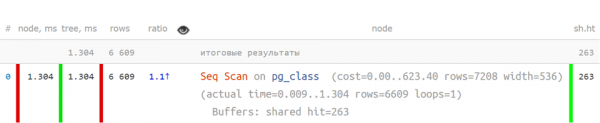
Is it easy to understand the plan when it looks like this?

Seq Scan on pg_class (actual time=0.009..1.304 rows=6609 loops=1)
  Buffers: shared hit=263
Planning Time: 0.108 ms
Execution Time: 1.800 ms

Not really.

But like this, in a shortened form,, when key indicators are separated, it becomes much clearer:

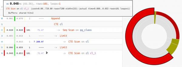
But if the plan is more complex, the pie chart of time distribution by nodes comes to the rescue:

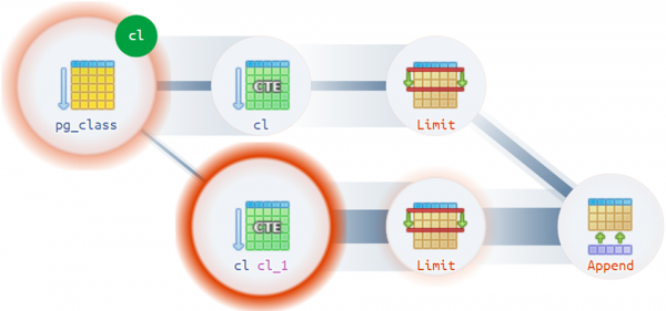
Well, for the most complex cases, the execution diagram:

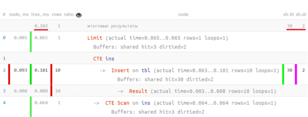
For example, there are quite non-trivial situations where a plan can have more than one actual root:

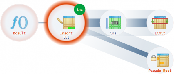
Structural hints

Well, if the entire structure of the plan and its pain points are already outlined and visible — why not highlight them for the developer and explain in "plain language"?

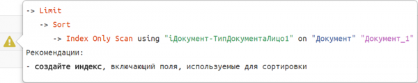We have already collected a couple of dozen such recommendation templates.

Row-level query profiler

Now, if you overlay the original query onto the analyzed plan, you can see how much time was spent on each individual operator — approximately like this:

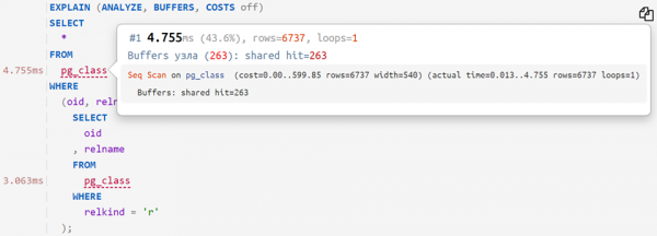
… or even like this:

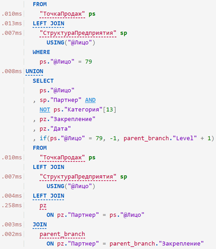
Parameter substitution in the query

If you have "attached" not only the query to the plan but also its parameters from the DETAIL line of the log, you can additionally copy it in one of the options:

with value substitution in the query
for direct execution on your database and further profiling
```
SELECT 'const', 'param'::text;
```
with value substitution through PREPARE/EXECUTE
to emulate the scheduler's operation when the parameter part can be ignored — for example, when working on partitioned tables
```
DEALLOCATE ALL;
PREPARE q(text) AS SELECT 'const', $1::text;
EXECUTE q('param'::text);
```