

The package tidyr is part of one of the most popular libraries in R language - tidyverse.
The main purpose of the package is to tidy data.
There is already dedicated to this package, but it dates back to 2015. I want to talk about the most relevant changes that its author Hadley Wickham announced just a few days ago.

SJK: Will the functions gather() and spread() be deprecated?
Hadley Wickham: To some extent. We will stop recommending the use of these functions and fixing bugs in them, but they will still remain in the package in their current state.
Content
If you're interested in data analysis, you might find my and channels interesting. Most of the content is dedicated to the R language.
The TidyData Concept
The goal tidyr — to help you tidy your data. Tidy data means data where:
- Every variable is in a column.
- Every observation is a row.
- Every value is a cell.
Data that is tidied to tidy data is significantly easier and more convenient to work with during analysis.
The main functions included in the tidyr package
tidyr contains a set of functions designed for table transformations:
fill()— fills in missing values in a column with the previous values;separate()— splits one field into several using a separator;unite()— performs the operation of combining several fields into one, the reverse action of the functionseparate();pivot_longer()— a function that transforms data from wide format to long;pivot_wider()— a function that transforms data from long format to wide. The reverse operation of what is performed by the functionpivot_longer().gather()deprecated — a function that transforms data from wide format to long;spread()deprecated — a function that transforms data from long format to wide. The reverse operation of what is performed by the functiongather().
A new concept for transforming data from wide format to long and vice versa
Previously, functions were used for such transformations gather() and spread()Over the years these functions have existed, it has become clear that for most users, including the package author, the names of these functions and their arguments were not very obvious, causing difficulties in finding and understanding which of these functions converts a data frame from wide to long format, and vice versa.
In this regard, tidyr two new, important functions have been added, designed for transforming data frames.
New features pivot_longer() and pivot_wider() were created under the influence of some functions from the package cdata, created by John Mount and Nina Zumel.
Installing the latest version of tidyr 0.8.3.9000
To install the new, most up-to-date version of the package, tidyr 0.8.3.9000, which includes the new functions, use the following code.
devtools::install_github("tidyverse/tidyr")
At the time of writing this article, these functions are only available in the dev version of the package on GitHub.
Transition to new functions
In fact, translating old scripts to work with new functions is not difficult; for better understanding, I will take an example from the documentation of the old functions and show how these same operations are performed using the new pivot_*() functions.
Converting wide format to long.
Example code from the gather function documentation
# example
library(dplyr)
stocks <- data.frame(
  time = as.Date('2009-01-01') + 0:9,
  X = rnorm(10, 0, 1),
  Y = rnorm(10, 0, 2),
  Z = rnorm(10, 0, 4)
)

# old
stocks_gather <- stocks %>% gather(key   = stock,
                                   value = price,
                                   -time)

# new
stocks_long   <- stocks %>% pivot_longer(cols      = -time,
                                       names_to  = "stock",
                                       values_to = "price")
Converting long format to wide.
Example code from the spread function documentation
# old
stocks_spread <- stocks_gather %>% spread(key = stock,
                                          value = price)

# new
stock_wide    <- stocks_long %>% pivot_wider(names_from  = "stock",
                                            values_from = "price")
Since the examples above work with pivot_longer() and pivot_wider(), in the original table stocks there are no columns listed in the arguments names_to and values_to their names must be specified in quotes.
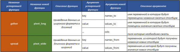
A table that will help you easily understand how to transition to working with the new concept tidyr.
Note from the Author
Everything presented in the following text is adaptive; I would even say a free translation of the from the official tidyverse library website.
A simple example of transforming data from wide format to long
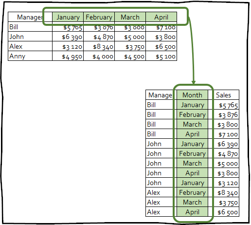
pivot_longer () — makes data sets longer by reducing the number of columns and increasing the number of rows.
To run the examples presented in the article, you need to first load the necessary packages:
library(tidyr)
library(dplyr)
library(readr)
Suppose we have a table with survey results, which (among other things) asked people about their religion and annual income:
#> # A tibble: 18 x 11
#>    religion `<$10k` `$10-20k` `$20-30k` `$30-40k` `$40-50k` `$50-75k`
#>    <chr>      <dbl>     <dbl>     <dbl>     <dbl>     <dbl>     <dbl>
#>  1 Agnostic      27        34        60        81        76       137
#>  2 Atheist       12        27        37        52        35        70
#>  3 Buddhist      27        21        30        34        33        58
#>  4 Catholic     418       617       732       670       638      1116
#>  5 Don’t k…      15        14        15        11        10        35
#>  6 Evangel…     575       869      1064       982       881      1486
#>  7 Hindu          1         9         7         9        11        34
#>  8 Histori…     228       244       236       238       197       223
#>  9 Jehovah…      20        27        24        24        21        30
#> 10 Jewish        19        19        25        25        30        95
#> # … with 8 more rows, and 4 more variables: `$75-100k` <dbl>,
#> #   `$100-150k` <dbl>, `>150k` <dbl>, `Don't know/refused` <dbl>
This table contains data on the respondents' religion in rows, while income levels are spread across the column names. The number of respondents from each category is stored in the cell values at the intersection of religion and income level. To tidy the table into a neat, correct format, simply use pivot_longer():
pew %>%
  pivot_longer(cols = -religion, names_to = "income", values_to = "count")
pew %>%
pivot_longer(cols = -religion, names_to = "income", values_to = "count")
#> # A tibble: 180 x 3
#> religion income count
#>
#> 1 Agnostic 2 Agnostic $10-20k 34
#> 3 Agnostic $20-30k 60
#> 4 Agnostic $30-40k 81
#> 5 Agnostic $40-50k 76
#> 6 Agnostic $50-75k 137
#> 7 Agnostic $75-100k 122
#> 8 Agnostic $100-150k 109
#> 9 Agnostic >150k 84
#> 10 Agnostic Don't know/refused 96
#> # … with 170 more rowsFunction arguments pivot_longer()
- The first argument cols, describes which columns need to be combined. In this case, all columns except time.
- Argument names_to gives the name of the variable that will be created from the names of the columns we combined.
- values_to gives the name of the variable that will be created from the data stored in the cell values of the combined columns.
Specifications
This is a new feature of the package tidyr, which was previously unavailable when working with deprecated functions.
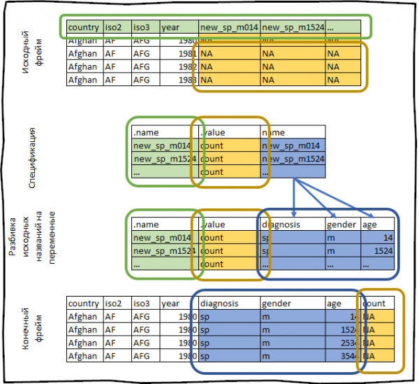
The specification is a data frame where each row corresponds to one column in the new output data frame, along with two special columns that start with:
- .name contains the original column name.
- .value contains the name of the column that will hold the cell values.
The remaining specification columns reflect how the names of the columns being compressed will appear in the new column from .name.
The specification describes metadata stored in the column name, with one row for each column and one column for each variable combined with the column name. This definition might seem confusing right now, but after looking at a few examples, it will become much clearer.
The essence of the specification is that you can extract, modify, and assign new metadata to the transformed data frame.
To work with specifications when transforming a table from wide format to long format, the function used is pivot_longer_spec().
How this function works is that it takes any data frame and forms its metadata in the way described above.
For example, let's take the who dataset that comes with the package. tidyrThis dataset contains information provided by the World Health Organization about tuberculosis incidence.
who
#> # A tibble: 7,240 x 60
#>    country iso2  iso3   year new_sp_m014 new_sp_m1524 new_sp_m2534
#>        & &
#>  1 Afghan… AF    AFG    1980          NA           NA           NA
#>  2 Afghan… AF    AFG    1981          NA           NA           NA
#>  3 Afghan… AF    AFG    1982          NA           NA           NA
#>  4 Afghan… AF    AFG    1983          NA           NA           NA
#>  5 Afghan… AF    AFG    1984          NA           NA           NA
#>  6 Afghan… AF    AFG    1985          NA           NA           NA
#>  7 Afghan… AF    AFG    1986          NA           NA           NA
#>  8 Afghan… AF    AFG    1987          NA           NA           NA
#>  9 Afghan… AF    AFG    1988          NA           NA           NA
#> 10 Afghan… AF    AFG    1989          NA           NA           NA
#> # … with 7,230 more rows, and 53 more variables
We will build its specification.
spec %
  pivot_longer_spec(new_sp_m014:newrel_f65, values_to = "count")
#> # A tibble: 56 x 3
#> .name .value name
#> <chr> <chr> <chr>
#> 1 new_sp_m014 count new_sp_m014
#> 2 new_sp_m1524 count new_sp_m1524
#> 3 new_sp_m2534 count new_sp_m2534
#> 4 new_sp_m3544 count new_sp_m3544
#> 5 new_sp_m4554 count new_sp_m4554
#> 6 new_sp_m5564 count new_sp_m5564
#> 7 new_sp_m65 count new_sp_m65
#> 8 new_sp_f014 count new_sp_f014
#> 9 new_sp_f1524 count new_sp_f1524
#> 10 new_sp_f2534 count new_sp_f2534
#> # … with 46 more rowsFields country, iso2, iso3 are already variables. Our task is to pivot the columns with new_sp_m014 by newrel_f65.
The names of these columns contain the following information:
- The prefix
new_indicates that the column contains data on new tuberculosis cases; the current data frame contains information only on new cases, so this prefix has no semantic meaning in the current context. sp/rel/sp/epdescribes the method of disease diagnosis.m/fthe patient's gender.014/1524/2535/3544/4554/65the patient's age range.
We can separate these columns using the function extract(), using a regular expression.
spec %
        extract(name, c("diagnosis", "gender", "age"), "new_?(.*)_(.)(.*)")
#> # A tibble: 56 x 5
#> .name .value diagnosis gender age
#> <chr> <chr> <chr> <chr> <chr>
#> 1 new_sp_m014 count sp m 014
#> 2 new_sp_m1524 count sp m 1524
#> 3 new_sp_m2534 count sp m 2534
#> 4 new_sp_m3544 count sp m 3544
#> 5 new_sp_m4554 count sp m 4554
#> 6 new_sp_m5564 count sp m 5564
#> 7 new_sp_m65 count sp m 65
#> 8 new_sp_f014 count sp f 014
#> 9 new_sp_f1524 count sp f 1524
#> 10 new_sp_f2534 count sp f 2534
#> # … with 46 more rowsNote, the column .name should remain unchanged, as it is our index in the names of the original dataset's columns.
Gender and age (the columns gender and age) have fixed and known values, so it is advisable to convert these columns to factors:
spec %
            mutate(
              gender = factor(gender, levels = c("f", "m")),
              age = factor(age, levels = unique(age), ordered = TRUE)
            )
Finally, to apply the specification we created to the original data frame who we need to use the argument spec in the function pivot_longer().
who %>% pivot_longer(spec = spec)
#> # A tibble: 405,440 x 8
#>    country     iso2  iso3   year diagnosis gender age   count
#>    <chr>       <chr> <chr> <int> <chr>     <fct>  <ord> <int>
#>  1 Afghanistan AF    AFG    1980 sp        m      014      NA
#>  2 Afghanistan AF    AFG    1980 sp        m      1524     NA
#>  3 Afghanistan AF    AFG    1980 sp        m      2534     NA
#>  4 Afghanistan AF    AFG    1980 sp        m      3544     NA
#>  5 Afghanistan AF    AFG    1980 sp        m      4554     NA
#>  6 Afghanistan AF    AFG    1980 sp        m      5564     NA
#>  7 Afghanistan AF    AFG    1980 sp        m      65       NA
#>  8 Afghanistan AF    AFG    1980 sp        f      014      NA
#>  9 Afghanistan AF    AFG    1980 sp        f      1524     NA
#> 10 Afghanistan AF    AFG    1980 sp        f      2534     NA
#> # … with 405,430 more rows
Everything we've just done can be illustrated as follows:
Specification using multiple values (.value)
In the example above, the specification column .value contained only one value, which is usually the case.
But occasionally a situation may arise where you need to combine data from columns of different data types. With the outdated function, spread() it would be quite difficult to do this.
The example given below is taken from the package data.table.
Let's create a practice dataframe.
family <- tibble::tribble(
  ~family,  ~dob_child1,  ~dob_child2, ~gender_child1, ~gender_child2,
       1L, "1998-11-26", "2000-01-29",             1L,             2L,
       2L, "1996-06-22",           NA,             2L,             NA,
       3L, "2002-07-11", "2004-04-05",             2L,             2L,
       4L, "2004-10-10", "2009-08-27",             1L,             1L,
       5L, "2000-12-05", "2005-02-28",             2L,             1L,
)
family % mutate_at(vars(starts_with("dob")), parse_date)
#> # A tibble: 5 x 5
#> family dob_child1 dob_child2 gender_child1 gender_child2
#> <int> <date> <date> <int> <int>
#> 1 1 1998-11-26 2000-01-29 1 2
#> 2 2 1996-06-22 NA 2 NA
#> 3 3 2002-07-11 2004-04-05 2 2
#> 4 4 2004-10-10 2009-08-27 1 1
#> 5 5 2000-12-05 2005-02-28 2 1The created dataframe contains data about the children of one family in each row. Families may have one or two children. For each child, information about their date of birth and gender is provided, with the data for each child in separate columns. Our task is to bring this data to a format suitable for analysis.
Note that we have two variables with information about each child: their gender and date of birth (the columns with the prefix dob contain the date of birth, while the columns with the prefix gender contain the child's gender). In the expected result, they should be in separate columns. We can achieve this by generating a specification in which the column .value will have two different values.
spec %
  pivot_longer_spec(-family) %>%
  separate(col = name, into = c(".value", "child")) %>%
  mutate(child = parse_number(child))
#> # A tibble: 4 x 3
#>   .name         .value child
#>   <chr>         <chr>  <dbl>
#> 1 dob_child1    dob        1
#> 2 dob_child2    dob        2
#> 3 gender_child1 gender     1
#> 4 gender_child2 gender     2
So, let's break down the steps that the above code executes.
pivot_longer_spec(-family)— we create a specification that compresses all existing columns except the family column.separate(col = name, into = c(".value", "child"))— we split the column .name, which contains the names of the original fields, by underscore and place the resulting values into the columns .value and child.mutate(child = parse_number(child))— we convert the field values child from text to numeric data type.
Now we can apply the obtained specification to the original dataframe and bring the table to the desired form.
family %>%
    pivot_longer(spec = spec, na.rm = T)
#> # A tibble: 9 x 4
#> family child dob gender
#> <int> <dbl> <date> <int>
#> 1 1 1 1998-11-26 1
#> 2 1 2 2000-01-29 2
#> 3 2 1 1996-06-22 2
#> 4 3 1 2002-07-11 2
#> 5 3 2 2004-04-05 2
#> 6 4 1 2004-10-10 1
#> 7 4 2 2009-08-27 1
#> 8 5 1 2000-12-05 2
#> 9 5 2 2005-02-28 1We use the argument na.rm = TRUE, because the current form of the data forces us to create extra rows for non-existent observations. Since family 2 has only one child, na.rm = TRUE ensures that family 2 will have one row in the output.
Transforming data frames from long format to wide
pivot_wider() is the inverse transformation, and conversely increases the number of columns in the data frame by reducing the number of rows.
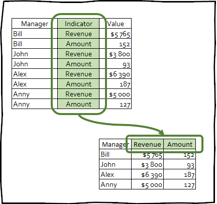
Such transformations are rarely used to clean data, yet this technique can be useful for creating summary tables for presentations or for integration with other tools.
In fact, the functions pivot_longer() and pivot_wider() are symmetrical and perform inverse actions on each other, i.e.: df %>% pivot_longer(spec = spec) %>% pivot_wider(spec = spec) and df %>% pivot_wider(spec = spec) %>% pivot_longer(spec = spec) will return the original df.
A basic example of tidying a table to a wide format
To demonstrate how the function works, pivot_wider() we will use the dataset fish_encounters, which contains information on how various stations track the movement of fish in the river.
#> # A tibble: 114 x 3
#>    fish  station  seen
#>    <fct> <fct>   <int>
#>  1 4842  Release     1
#>  2 4842  I80_1       1
#>  3 4842  Lisbon      1
#>  4 4842  Rstr        1
#>  5 4842  Base_TD     1
#>  6 4842  BCE         1
#>  7 4842  BCW         1
#>  8 4842  BCE2        1
#>  9 4842  BCW2        1
#> 10 4842  MAE         1
#> # … with 104 more rows
In most cases, this table will be more informative and convenient to use if the information for each station is presented in a separate column.
fish_encounters %>% pivot_wider(names_from = station, values_from = seen)
fish_encounters %>% pivot_wider(names_from = station, values_from = seen)
#> # A tibble: 19 x 12
#>    fish  Release I80_1 Lisbon  Rstr Base_TD   BCE   BCW  BCE2  BCW2   MAE
#>        &   &    & & & & &
#>  1 4842        1     1      1     1       1     1     1     1     1     1
#>  2 4843        1     1      1     1       1     1     1     1     1     1
#>  3 4844        1     1      1     1       1     1     1     1     1     1
#>  4 4845        1     1      1     1       1    NA    NA    NA    NA    NA
#>  5 4847        1     1      1    NA      NA    NA    NA    NA    NA    NA
#>  6 4848        1     1      1     1      NA    NA    NA    NA    NA    NA
#>  7 4849        1     1     NA    NA      NA    NA    NA    NA    NA    NA
#>  8 4850        1     1     NA     1       1     1     1    NA    NA    NA
#>  9 4851        1     1     NA    NA      NA    NA    NA    NA    NA    NA
#> 10 4854        1     1     NA    NA      NA    NA    NA    NA    NA    NA
#> # … with 9 more rows, and 1 more variable: MAW
This dataset records information only in cases where a fish was detected by the station, meaning that if any fish were not recorded by some station, that data will not be in the table. This implies that the output will be filled with NA.
However, in this case, we know that the absence of a record means that the fish was not observed, so we can use the argument values_fill in the function pivot_wider() and fill these missing values with zeros:
fish_encounters %>% pivot_wider(
  names_from = station,
  values_from = seen,
  values_fill = list(seen = 0)
)
#> # A tibble: 19 x 12
#> fish Release I80_1 Lisbon Rstr Base_TD BCE BCW BCE2 BCW2 MAE
#> <fct> <int> <int> <int> <int> <int> <int> <int> <int> <int> <int>
#> 1 4842 1 1 1 1 1 1 1 1 1 1
#> 2 4843 1 1 1 1 1 1 1 1 1 1
#> 3 4844 1 1 1 1 1 1 1 1 1 1
#> 4 4845 1 1 1 1 1 0 0 0 0 0
#> 5 4847 1 1 1 0 0 0 0 0 0 0
#> 6 4848 1 1 1 1 0 0 0 0 0 0
#> 7 4849 1 1 0 0 0 0 0 0 0 0
#> 8 4850 1 1 0 1 1 1 1 0 0 0
#> 9 4851 1 1 0 0 0 0 0 0 0 0
#> 10 4854 1 1 0 0 0 0 0 0 0 0
#> # … with 9 more rows, and 1 more variable: MAW <int>Generating a column name from several source variables
Imagine that we have a table containing combinations of product, country, and year. You can generate a test data frame using the following code:
df %
  filter((product == "A" & country == "AI") | product == "B") %>%
  mutate(value = rnorm(nrow(.)))
#> # A tibble: 45 x 4
#> product country year value
#> <chr> <chr> <int> <dbl>
#> 1 A AI 2000 -2.05
#> 2 A AI 2001 -0.676
#> 3 A AI 2002 1.60
#> 4 A AI 2003 -0.353
#> 5 A AI 2004 -0.00530
#> 6 A AI 2005 0.442
#> 7 A AI 2006 -0.610
#> 8 A AI 2007 -2.77
#> 9 A AI 2008 0.899
#> 10 A AI 2009 -0.106
#> # … with 35 more rowsOur task is to expand the data frame so that one column contains data for each combination of product and country. To do this, it's sufficient to pass to the argument names_from a vector containing the names of the fields to be combined.
df %>% pivot_wider(names_from = c(product, country),
                 values_from = "value")
#> # A tibble: 15 x 4
#> year A_AI B_AI B_EI
#> <int> <dbl> <dbl> <dbl>
#> 1 2000 -2.05 0.607 1.20
#> 2 2001 -0.676 1.65 -0.114
#> 3 2002 1.60 -0.0245 0.501
#> 4 2003 -0.353 1.30 -0.459
#> 5 2004 -0.00530 0.921 -0.0589
#> 6 2005 0.442 -1.55 0.594
#> 7 2006 -0.610 0.380 -1.28
#> 8 2007 -2.77 0.830 0.637
#> 9 2008 0.899 0.0175 -1.30
#> 10 2009 -0.106 -0.195 1.03
#> # … with 5 more rowsYou can also apply specifications to the function pivot_wider(). But when passed to pivot_wider() the specification performs the opposite transformation pivot_longer(): it creates columns as specified in .name, using values from .value and other columns.
For this dataset, you can generate a custom specification if you want every possible combination of country and product to have its own column, not just those present in the data:
spec %
  expand(product, country, .value = "value") %>%
  unite(".name", product, country, remove = FALSE)
#> # A tibble: 4 x 4
#> .name product country .value
#> <chr> <chr> <chr> <chr>
#> 1 A_AI A AI value
#> 2 A_EI A EI value
#> 3 B_AI B AI value
#> 4 B_EI B EI valuedf %>% pivot_wider(spec = spec) %>% head()#> # A tibble: 6 x 5
#> year A_AI A_EI B_AI B_EI
#> <int> <dbl> <dbl> <dbl> <dbl>
#> 1 2000 -2.05 NA 0.607 1.20
#> 2 2001 -0.676 NA 1.65 -0.114
#> 3 2002 1.60 NA -0.0245 0.501
#> 4 2003 -0.353 NA 1.30 -0.459
#> 5 2004 -0.00530 NA 0.921 -0.0589
#> 6 2005 0.442 NA -1.55 0.594Several advanced examples of working with the new tidyr concept
Tidying data using a dataset on income and rent census in the USA
Dataset us_rent_income contains information about the average income and rent for each state in the USA for 2017 (the dataset is available in the package tidycensus).
us_rent_income
#> # A tibble: 104 x 5
#>    GEOID NAME       variable estimate   moe
#>
#>  1 01    Alabama    income      24476   136
#>  2 01    Alabama    rent          747     3
#>  3 02    Alaska     income      32940   508
#>  4 02    Alaska     rent         1200    13
#>  5 04    Arizona    income      27517   148
#>  6 04    Arizona    rent          972     4
#>  7 05    Arkansas   income      23789   165
#>  8 05    Arkansas   rent          709     5
#>  9 06    California income      29454   109
#> 10 06    California rent         1358     3
#> # … with 94 more rows
In the form in which the data is stored in the dataset, us_rent_income working with it is extremely inconvenient, so we would like to create a dataset with the columns: rent, rent_moe, come, income_moe. There are many ways to create this specification, but the main point is that we need to generate each combination of variable values and estimate/moe, and then generate the column name.
  spec %
    expand(variable, .value = c("estimate", "moe")) %>%
    mutate(
      .name = paste0(variable, ifelse(.value == "moe", "_moe", ""))
    )
#> # A tibble: 4 x 3
#> variable .value .name
#> <chr> <chr> <chr>
#> 1 income estimate income
#> 2 income moe income_moe
#> 3 rent estimate rent
#> 4 rent moe rent_moeProviding this specification pivot_wider() gives us the result we are looking for:
us_rent_income %>% pivot_wider(spec = spec)
#> # A tibble: 52 x 6
#>    GEOID NAME                 income income_moe  rent rent_moe
#>    <chr> <chr>                 <dbl>      <dbl> <dbl>    <dbl>
#>  1 01    Alabama               24476        136   747        3
#>  2 02    Alaska                32940        508  1200       13
#>  3 04    Arizona               27517        148   972        4
#>  4 05    Arkansas              23789        165   709        5
#>  5 06    California            29454        109  1358        3
#>  6 08    Colorado              32401        109  1125        5
#>  7 09    Connecticut           35326        195  1123        5
#>  8 10    Delaware              31560        247  1076       10
#>  9 11    District of Columbia  43198        681  1424       17
#> 10 12    Florida               25952         70  1077        3
#> # … with 42 more rows
World Bank
Sometimes transforming a dataset into the required format involves several steps.
Dataset world_bank_pop contains data from the World Bank on the population of each country from 2000 to 2018.
#> # A tibble: 1,056 x 20
#>    country indicator `2000` `2001` `2002` `2003`  `2004`  `2005`   `2006`
#>    <chr>   <chr>      <dbl>  <dbl>  <dbl>  <dbl>   <dbl>   <dbl>    <dbl>
#>  1 ABW     SP.URB.T… 4.24e4 4.30e4 4.37e4 4.42e4 4.47e+4 4.49e+4  4.49e+4
#>  2 ABW     SP.URB.G… 1.18e0 1.41e0 1.43e0 1.31e0 9.51e-1 4.91e-1 -1.78e-2
#>  3 ABW     SP.POP.T… 9.09e4 9.29e4 9.50e4 9.70e4 9.87e+4 1.00e+5  1.01e+5
#>  4 ABW     SP.POP.G… 2.06e0 2.23e0 2.23e0 2.11e0 1.76e+0 1.30e+0  7.98e-1
#>  5 AFG     SP.URB.T… 4.44e6 4.65e6 4.89e6 5.16e6 5.43e+6 5.69e+6  5.93e+6
#>  6 AFG     SP.URB.G… 3.91e0 4.66e0 5.13e0 5.23e0 5.12e+0 4.77e+0  4.12e+0
#>  7 AFG     SP.POP.T… 2.01e7 2.10e7 2.20e7 2.31e7 2.41e+7 2.51e+7  2.59e+7
#>  8 AFG     SP.POP.G… 3.49e0 4.25e0 4.72e0 4.82e0 4.47e+0 3.87e+0  3.23e+0
#>  9 AGO     SP.URB.T… 8.23e6 8.71e6 9.22e6 9.77e6 1.03e+7 1.09e+7  1.15e+7
#> 10 AGO     SP.URB.G… 5.44e0 5.59e0 5.70e0 5.76e0 5.75e+0 5.69e+0  4.92e+0
#> # … with 1,046 more rows, and 11 more variables: `2007` <dbl>,
#> #   `2008` <dbl>, `2009` <dbl>, `2010` <dbl>, `2011` <dbl>, `2012` <dbl>,
#> #   `2013` <dbl>, `2014` <dbl>, `2015` <dbl>, `2016` <dbl>, `2017` <dbl>
Our goal is to create a tidy dataset where each variable is in its own column. It's currently unclear what specific steps are necessary, but we will start with the most obvious issue: the year is spread across multiple columns.
To fix this, we need to use the function pivot_longer().
pop2 %
  pivot_longer(`2000`:`2017`, names_to = "year")
#> # A tibble: 19,008 x 4
#> country indicator year value
#> <chr> <chr> <chr> <dbl>
#> 1 ABW SP.URB.TOTL 2000 42444
#> 2 ABW SP.URB.TOTL 2001 43048
#> 3 ABW SP.URB.TOTL 2002 43670
#> 4 ABW SP.URB.TOTL 2003 44246
#> 5 ABW SP.URB.TOTL 2004 44669
#> 6 ABW SP.URB.TOTL 2005 44889
#> 7 ABW SP.URB.TOTL 2006 44881
#> 8 ABW SP.URB.TOTL 2007 44686
#> 9 ABW SP.URB.TOTL 2008 44375
#> 10 ABW SP.URB.TOTL 2009 44052
#> # … with 18,998 more rowsThe next step is to consider the variable indicator.
pop2 %>% count(indicator)
#> # A tibble: 4 x 2
#>   indicator       n
#>   <chr>       <int>
#> 1 SP.POP.GROW  4752
#> 2 SP.POP.TOTL  4752
#> 3 SP.URB.GROW  4752
#> 4 SP.URB.TOTL  4752
Where SP.POP.GROW is population growth, SP.POP.TOTL is total population, and SP.URB.* is the same, but only for urban areas. Let's separate these values into two variables: area (total or urban) and a variable containing the actual data (population or growth):
pop3 %
  separate(indicator, c(NA, "area", "variable"))
#> # A tibble: 19,008 x 5
#> country area variable year value
#> <chr> <chr> <chr> <chr> <dbl>
#> 1 ABW URB TOTL 2000 42444
#> 2 ABW URB TOTL 2001 43048
#> 3 ABW URB TOTL 2002 43670
#> 4 ABW URB TOTL 2003 44246
#> 5 ABW URB TOTL 2004 44669
#> 6 ABW URB TOTL 2005 44889
#> 7 ABW URB TOTL 2006 44881
#> 8 ABW URB TOTL 2007 44686
#> 9 ABW URB TOTL 2008 44375
#> 10 ABW URB TOTL 2009 44052
#> # … with 18,998 more rowsNow we just need to split the variable into two columns:
pop3 %>%
  pivot_wider(names_from = variable, values_from = value)
#> # A tibble: 9,504 x 5
#> country area year TOTL GROW
#> <chr> <chr> <chr> <dbl> <dbl>
#> 1 ABW URB 2000 42444 1.18
#> 2 ABW URB 2001 43048 1.41
#> 3 ABW URB 2002 43670 1.43
#> 4 ABW URB 2003 44246 1.31
#> 5 ABW URB 2004 44669 0.951
#> 6 ABW URB 2005 44889 0.491
#> 7 ABW URB 2006 44881 -0.0178
#> 8 ABW URB 2007 44686 -0.435
#> 9 ABW URB 2008 44375 -0.698
#> 10 ABW URB 2009 44052 -0.731
#> # … with 9,494 more rowsContact list
In the last example, imagine you have a list of contacts that you copied and pasted from a website:
contacts <- tribble(
  ~field, ~value,
  "name", "Jiena McLellan",
  "company", "Toyota",
  "name", "John Smith",
  "company", "google",
  "email", "john@google.com",
  "name", "Huxley Ratcliffe"
)
Transforming this list into a tabular format is quite challenging because there is no variable that identifies which data belongs to which contact. We can fix this by noting that the data for each new contact starts with a name ("name"). Therefore, we can create a unique identifier and increment it by one each time the value "name" appears in the field column:
contacts %
  mutate(
    person_id = cumsum(field == "name")
  )
contacts
#> # A tibble: 6 x 3
#> field value person_id
#> <chr> <chr> <int>
#> 1 name Jiena McLellan 1
#> 2 company Toyota 1
#> 3 name John Smith 2
#> 4 company google 2
#> 5 email john@google.com 2
#> 6 name Huxley Ratcliffe 3Now that we have a unique identifier for each contact, we can pivot the field and value into columns:
contacts %>%
  pivot_wider(names_from = field, values_from = value)
#> # A tibble: 3 x 4
#> person_id name company email
#> <int> <chr> <chr> <chr>
#> 1 1 Jiena McLellan Toyota <NA>
#> 2 2 John Smith google john@google.com
#> 3 3 Huxley Ratcliffe <NA> <NA>Conclusion
In my personal opinion, the new concept tidyr is indeed intuitively clearer and significantly outperforms outdated functions. spread() and gather(). I hope this article helped you understand pivot_longer() and pivot_wider().
Source: habr.com
