

Hello.
I've decided to share my discovery — the result of contemplation, trials, and errors.
Essentially, this is not really a discovery, of course — all of this should have been well-known to those engaged in applied statistical data processing and optimization of any systems, not necessarily just databases.
And yes, they know, they write interesting articles about their research. (UPD: in the comments, they pointed to a very interesting project: )
On the other hand, I don't see broad mention or distribution of such an approach on the internet among IT specialists and DBAs.
So, to the point.
Let's assume we have a task: to configure some service system to support a certain operation.
About this work — it is known: what it entails, how the quality of this work is measured, and what criteria are used to assess this quality.
Also, let's assume that it's more or less clear how this work is performed in (or with) this service system.
"More or less" means that there is an opportunity to prepare (or obtain somewhere) some tool, utility, or service that can generate and provide to the system a test load sufficiently adequate to what will be in production, under conditions reasonably close to those in production.
Well, let's say that the set of adjustable parameters of this service system is known, which can be used to configure this system in terms of its operational productivity.
And the problem is — there is not enough complete understanding of this service system, one that allows for expert configuration of this system for future load on this platform to achieve the required productivity of the system.
Well, this is usually how it goes.
What can be done here.
Well, the first thing that comes to mind is to check the documentation for this system. Understand what the acceptable ranges for the adjustable parameter values are. And, for example, using the coordinate descent method, adjust the values for the system parameters in tests.
That is, specify some configuration for the system, in the form of a specific set of values for its tuning parameters.
Apply a test load to it using this very tool-utility, load generator.
And observe the response time, or the quality metrics of the system's performance.
Another thought might be that — this could take a very long time.
So, that is: if there are many configuration parameters, if the ranges of their values are large, if each individual load test takes a long time to execute, then yes, this can take an unacceptably long time.
And here, what can be understood and remembered.
You can find out that in the set of values for the configuration parameters of the service system, there is a vector, like a sequence of values.
Each such vector, assuming other things are equal (in that this vector does not affect), corresponds to a quite definite value of the metric — a quality indicator of the system's performance under the test load.
That is,
Let's denote the configuration vector of the system as  , where
  ; where
  — the number of system configuration parameters, how many of these parameters there are.
And the value of the metric corresponding to this  we will denote as
 , so we get a function:
So then, everything immediately comes down to, in my case: almost forgotten since university days, algorithms for finding the extremum of a function.
Well, here arises an organizational and practical question: which specific algorithm to use.
- In the sense — so that I have to code as little as possible myself.
- And so that it works, i.e., finds the extremum (if there is one), at least — faster than coordinate descent.
The first point hints that we should look towards some environments where such algorithms are already implemented and are in some form ready to use in code.
Well, I know about python and cran-r
The second point indicates that I need to read about the algorithms themselves, what they are, their requirements, and operational features.
And what they provide, useful side effects/results, either directly from the algorithm itself.
Or these can be obtained from the results of the algorithm's work.
A lot depends on the input conditions here.
For example, if for some reason, you need to get a result faster, then you need to look towards gradient descent algorithms, choosing one of them.
Or, if time is not so important, one can use stochastic optimization methods, such as a genetic algorithm.
I propose to consider the operation of such an approach to system configuration selection using a genetic algorithm in the next, so to speak: lab work.
Initial:
- Let there be, as a service system:
oracle xe 18c - Let it serve transactional activity with the goal of achieving the highest possible throughput of the database, in transactions per second.
- Transactions can vary greatly in their nature of data handling and context of operation.
Let’s agree that these are transactions that do not process a large amount of tabular data.
In the sense that they do not generate more undo data than redo and do not process large percentages of rows in large tables.
These transactions change one row in a relatively large table, with a small number of indexes on that table.
In this scenario, the productivity of the database in processing transactions will, with the caveat, be determined by the quality of handling the redo data.
Caveat — if we are specifically discussing the settings of the database.
Because, generally, there may be, for example, transactional locks between SQL sessions, due to, the design of user interactions with tabular data and/or the table model.
These will, of course, adversely affect the TPS metric, and this will be an exogenous factor relative to the database: the tabular model and the data interactions were designed in such a way that locks arise.
Therefore, for the purity of the experiment, we will exclude this factor; I will clarify how exactly below.
- Let’s assume, for clarity, that 100% of the SQL commands submitted to the database are DML commands.
Let the characteristics of user interactions with the database remain the same in tests.
Namely: the number of SQL sessions, the tabular data, how the SQL sessions interact with them. - The database operates in
FORCE LOGGING,ARCHIVELOGmodes. Flashback database mode is disabled at the database level. - Redo logs: located in a separate file system, on a separate 'disk';
All other parts of the physical component of the database: in another, separate file system, on a separate 'disk':
More details about the structure of the physical component of the lab database.
SQL> select status||' '||name from v$controlfile;
 /db/u14/oradata/XE/control01.ctl
SQL> select GROUP#||' '||MEMBER from v$logfile;
1 /db/u02/oradata/XE/redo01_01.log
2 /db/u02/oradata/XE/redo02_01.log
SQL> select FILE_ID||' '||TABLESPACE_NAME||' '||round(BYTES/1024/1024,2)||' '||FILE_NAME as col from dba_data_files;
4 UNDOTBS1 2208 /db/u14/oradata/XE/undotbs1_01.dbf
2 SLOB 128 /db/u14/oradata/XE/slob01.dbf
7 USERS 5 /db/u14/oradata/XE/users01.dbf
1 SYSTEM 860 /db/u14/oradata/XE/system01.dbf
3 SYSAUX 550 /db/u14/oradata/XE/sysaux01.dbf
5 MONITOR 128 /db/u14/oradata/XE/monitor.dbf
SQL> !cat /proc/mounts | egrep "/db/u[0-2]"
/dev/vda1 /db/u14 ext4 rw,noatime,nodiratime,data=ordered 0 0
/dev/mapper/vgsys-ora_redo /db/u02 xfs rw,noatime,nodiratime,attr2,nobarrier,inode64,logbsize=256k,noquota 0 0
Initially, I wanted to use a transaction-based database management system under these load conditions.
It has this wonderful feature, I will quote the author:
At the heart of SLOB is the 'SLOB method.' The SLOB Method aims to test platforms
without application contention. One cannot drive maximum hardware performance
using application code that is, for example, bound by application locking or even
sharing Oracle Database blocks. That's right—there is overhead when sharing data
in data blocks! But SLOB—in its default deployment—is immune to such contention.
This declaration: it corresponds, and so it is.
It is convenient to regulate the degree of parallelism of SQL sessions, this is the key -t to launching the utility. runit.sh from the SLOB suite.
It controls the percentage of DML commands in the number of SQL statements that are sent to the DB; each SQL session has the parameter UPDATE_PCT.
Separately and very conveniently: SLOB itself, before and after the load session—prepares statspack or AWR snapshots (whichever is specified to prepare).
However, it turned out that SLOB it does not support SQL sessions with a duration of less than 30 seconds.
So first, I coded my own, working-class version of the loader, and then it remained in use.
I will clarify about the loader—what it does and how, for clarity.
Essentially, the loader looks like this:
Worker code:
function dotx()
{
local v_period="$2"
[ -z "v_period" ] && v_period="0"
source "/home/oracle/testingredotrace/config.conf"

$ORACLE_HOME/bin/sqlplus -S system/${v_system_pwd} << __EOF__
whenever sqlerror exit failure
set verify off
set echo off
set feedback off

define wnum="$1"
define period="$v_period"
set appinfo worker_&&wnum

declare
 v_upto number;
 v_key  number;
 v_tots number;
 v_cts  number;
begin
 select max(col1) into v_upto from system.testtab_&&wnum;
 SELECT (( SYSDATE - DATE '1970-01-01' ) * 86400 ) into v_cts FROM DUAL;
 v_tots := &&period + v_cts;
 while v_cts <= v_tots
 loop
  v_key:=abs(mod(dbms_random.random,v_upto));
  if v_key=0 then
   v_key:=1;
  end if;
  update system.testtab_&&wnum t
  set t.object_name=translate(dbms_random.string('a', 120), 'abcXYZ', '158249')
  where t.col1=v_key
  ;
  commit;
  SELECT (( SYSDATE - DATE '1970-01-01' ) * 86400 ) into v_cts FROM DUAL;
 end loop;
end;
/

exit
__EOF__
}
export -f dotx
Workers are launched in the following way:
Launching workers.
echo "starting test, duration: ${TEST_DURATION}" >> "$v_logfile"
for((i=1;i> "$v_logfile"
 dotx "$i" "${TEST_DURATION}" &
done
echo "waiting..." >> "$v_logfile"
wait
The tables for workers are prepared as follows:
Creating tables
function createtable() {
source "/home/oracle/testingredotracе/config.conf"
$ORACLE_HOME/bin/sqlplus -S system/${v_system_pwd} << __EOF__
whenever sqlerror continue
set verify off
set echo off
set feedback off

define wnum="$1"
define ts_name="slob"

begin
 execute immediate 'drop table system.testtab_&&wnum';
exception when others then null;
end;
/

create table system.testtab_&&wnum tablespace &&ts_name as
select rownum as col1, t.*
from sys.dba_objects t
where rownum> "$v_logfile"
That is, for each worker (practically: a separate SQL session in the database), a separate table is created, with which the worker operates.
This achieves the absence of transaction locks between SQL sessions of the workers.
Each worker does the same thing with its table; all tables are identical.
All workers perform work for the same amount of time.
Moreover, it is sufficiently long to ensure that, for example, a log switch definitely occurs, and not just once.
Thus, related costs and effects arise.
In my case, I configured the duration of the workers' operation to 8 minutes.
A piece of the statspack report, describing the database operation under load.
Database    DB Id    Instance     Inst Num  Startup Time   Release     RAC
~~~~~~~~ ----------- ------------ -------- --------------- ----------- ---
          2929910313 XE                  1 07-Sep-20 23:12 18.0.0.0.0  NO

Host Name             Platform                CPUs Cores Sockets   Memory (G)
~~~~ ---------------- ---------------------- ----- ----- ------- ------------
     billing.izhevsk1 Linux x86 64-bit           2     2       1         15.6

Snapshot       Snap Id     Snap Time      Sessions Curs/Sess Comment
~~~~~~~~    ---------- ------------------ -------- --------- ------------------
Begin Snap:       1630 07-Sep-20 23:12:27       55        .7
  End Snap:       1631 07-Sep-20 23:20:29       62        .6
   Elapsed:       8.03 (mins) Av Act Sess:       8.4
   DB time:      67.31 (mins)      DB CPU:      15.01 (mins)

Cache Sizes            Begin        End
~~~~~~~~~~~       ---------- ----------
    Buffer Cache:     1,392M              Std Block Size:         8K
     Shared Pool:       288M                  Log Buffer:   103,424K

Load Profile              Per Second    Per Transaction    Per Exec    Per Call
~~~~~~~~~~~~      ------------------  ----------------- ----------- -----------
      DB time(s):                8.4                0.0        0.00        0.20
       DB CPU(s):                1.9                0.0        0.00        0.04
       Redo size:        7,685,765.6              978.4
   Logical reads:           60,447.0                7.7
   Block changes:           47,167.3                6.0
  Physical reads:                8.3                0.0
 Physical writes:              253.4                0.0
      User calls:               42.6                0.0
          Parses:               23.2                0.0
     Hard parses:                1.2                0.0
W/A MB processed:                1.0                0.0
          Logons:                0.5                0.0
        Executes:           15,756.5                2.0
       Rollbacks:                0.0                0.0
    Transactions:            7,855.1
Returning to the laboratory work assignment.
We will vary the values of such parameters of the laboratory database, assuming other factors are equal:
- Size of database log groups. Value range: [32, 1024] MB;
- Number of database log groups. Value range: [2, 32];
log_archive_max_processesvalue range: [1, 8];commit_loggingtwo values are allowed:batch|immediate;commit_waittwo values are allowed:wait|nowait;log_buffervalue range: [2, 128] MB.log_checkpoint_timeoutvalue range: [60, 1200] secondsdb_writer_processesvalue range: [1, 4]undo_retentionvalue range: [30, 300] secondstransactions_per_rollback_segmentvalue range: [1, 8]disk_asynch_iotwo values are allowed:true|false;filesystemio_optionsthe following values are allowed:none|setall|directIO|asynch;db_block_checkingthe following values are allowed:OFF|LOW|MEDIUM|FULL;db_block_checksumthe following values are allowed:OFF|TYPICAL|FULL;
An individual with experience in supporting Oracle databases can certainly say right now what values should be set for the parameters mentioned above to achieve better database performance for the data operations defined in the application code here.
But.
The purpose of the lab work is to show that the optimization algorithm will clarify this for us both efficiently and relatively quickly.
All we need to do is look at the documentation for the configurable system, just enough to determine which parameters to change and within what ranges.
Additionally, we need to code the solution that will implement the work with the configurable system of the chosen optimization algorithm.
Thus, now let’s discuss the code.
I mentioned above cran-r, meaning that all manipulations with the configurable system are orchestrated in the form of an R script.
The actual task, analysis, selection based on the metric values, and the state vectors of the system are encapsulated in the package GA ()
The package, in this case, is not very suitable, as it expects the task for the vectors (chromosomes, in the terms of the package) to be represented as a set of continuous numbers.
My vector, consisting of the values of the tuning parameters, comprises 14 variables — whole numbers and string values.
The issue can easily be circumvented by assigning specific numbers to the string values.
Thus, in the end, the main part of the R script looks like this:
Call GA::ga
cat( "", file=v_logfile, sep="n", append=F)

pSize = 10
elitism_value=1
pmutation_coef=0.8
pcrossover_coef=0.1
iterations=50

gam=GA::ga(type="real-valued", fitness=evaluate,
lower=c(32,2, 1,1,1,2,60,1,30,1,0,0, 0,0), upper=c(1024,32, 8,10,10,128,800,4,300,8,10,40, 40,30),
popSize=pSize,
pcrossover = pcrossover_coef,
pmutation = pmutation_coef,
maxiter=iterations,
run=4,
keepBest=T)
cat( "GA-session is done" , file=v_logfile, sep="n", append=T)
gam@solution
Here, using lower and upper attributes of the subprogram ga the search space is essentially defined within which a search will be conducted for a vector (or vectors) that will yield the maximum value of the fitness function.
The ga subprogram performs the search by maximizing the fitness function.
Thus, it turns out that in this case, the fitness function must interpret the vector as a set of values for specific database parameters, yielding metrics from the database.
That is, how many transactions per second does the database process given the current configuration and load on the database.
In other words, it needs to execute a multi-step process inside the fitness function:
- Processing the input vector of numbers — transforming it into values for the database parameters.
- Attempting to create the specified number of redo groups, of the specified size. Moreover, the attempt may not be successful.
Existing journal groups in the database, of some quantity and size, should be removed for experimental purity. - If the previous step is successful: configure the base values of the configuration parameters (again: there may be a failure).
- If the previous step is successful: stop the database, and restart it so that the newly set parameter values take effect. (again: there may be a failure).
- If the previous step is successful: perform a load test and obtain metrics from the database.
- Return the database to its original state, i.e., remove additional journal groups and restore the original database configuration.
Fitness function code
evaluate=function(p_par) {
v_module="evaluate"
v_metric=0
opn=NULL
opn$rg_size=round(p_par[1],digit=0)
opn$rg_count=round(p_par[2],digit=0)
opn$log_archive_max_processes=round(p_par[3],digit=0)
opn$commit_logging="BATCH"
if ( round(p_par[4],digit=0) > 5 ) {
 opn$commit_logging="IMMEDIATE"
}
opn$commit_logging=paste("'", opn$commit_logging, "'",sep="")

opn$commit_wait="WAIT"
if ( round(p_par[5],digit=0) > 5 ) {
 opn$commit_wait="NOWAIT"
}
opn$commit_wait=paste("'", opn$commit_wait, "'",sep="")

opn$log_buffer=paste(round(p_par[6],digit=0),"m",sep="")
opn$log_checkpoint_timeout=round(p_par[7],digit=0)
opn$db_writer_processes=round(p_par[8],digit=0)
opn$undo_retention=round(p_par[9],digit=0)
opn$transactions_per_rollback_segment=round(p_par[10],digit=0)
opn$disk_asynch_io="true"
if ( round(p_par[11],digit=0) > 5 ) {
 opn$disk_asynch_io="false"
}

opn$filesystemio_options="none"
if ( round(p_par[12],digit=0) > 10 && round(p_par[12],digit=0)  20 && round(p_par[12],digit=0)  30 ) {
 opn$filesystemio_options="asynch"
}

opn$db_block_checking="OFF"
if ( round(p_par[13],digit=0) > 10 && round(p_par[13],digit=0)  20 && round(p_par[13],digit=0)  30 ) {
 opn$db_block_checking="FULL"
}

opn$db_block_checksum="OFF"
if ( round(p_par[14],digit=0) > 10 && round(p_par[14],digit=0)  20 ) {
 opn$db_block_checksum="FULL"
}

v_vector=paste(round(p_par[1],digit=0),round(p_par[2],digit=0),round(p_par[3],digit=0),round(p_par[4],digit=0),round(p_par[5],digit=0),round(p_par[6],digit=0),round(p_par[7],digit=0),round(p_par[8],digit=0),round(p_par[9],digit=0),round(p_par[10],digit=0),round(p_par[11],digit=0),round(p_par[12],digit=0),round(p_par[13],digit=0),round(p_par[14],digit=0),sep=";")
cat( paste(v_module," try to evaluate vector: ", v_vector,sep="") , file=v_logfile, sep="n", append=T)

rc=make_additional_rgroups(opn)
if ( rc!=0 ) {
 cat( paste(v_module,"make_additional_rgroups failed",sep="") , file=v_logfile, sep="n", append=T)
 return (0)
}

v_rc=0
rc=set_db_parameter("log_archive_max_processes", opn$log_archive_max_processes)
if ( rc != 0 ) {  v_rc=1 }
rc=set_db_parameter("commit_logging", opn$commit_logging )
if ( rc != 0 ) {  v_rc=1 }
rc=set_db_parameter("commit_wait", opn$commit_wait )
if ( rc != 0 ) {  v_rc=1 }
rc=set_db_parameter("log_buffer", opn$log_buffer )
if ( rc != 0 ) {  v_rc=1 }
rc=set_db_parameter("log_checkpoint_timeout", opn$log_checkpoint_timeout )
if ( rc != 0 ) {  v_rc=1 }
rc=set_db_parameter("db_writer_processes", opn$db_writer_processes )
if ( rc != 0 ) {  v_rc=1 }
rc=set_db_parameter("undo_retention", opn$undo_retention )
if ( rc != 0 ) {  v_rc=1 }
rc=set_db_parameter("transactions_per_rollback_segment", opn$transactions_per_rollback_segment )
if ( rc != 0 ) {  v_rc=1 }
rc=set_db_parameter("disk_asynch_io", opn$disk_asynch_io )
if ( rc != 0 ) {  v_rc=1 }
rc=set_db_parameter("filesystemio_options", opn$filesystemio_options )
if ( rc != 0 ) {  v_rc=1 }
rc=set_db_parameter("db_block_checking", opn$db_block_checking )
if ( rc != 0 ) {  v_rc=1 }
rc=set_db_parameter("db_block_checksum", opn$db_block_checksum )
if ( rc != 0 ) {  v_rc=1 }

if ( rc!=0 ) {
 cat( paste(v_module," can not startup db with that vector of settings",sep="") , file=v_logfile, sep="n", append=T)
 rc=stop_db("immediate")
 rc=create_spfile()
 rc=start_db("")
 rc=remove_additional_rgroups(opn)
 return (0)
}

rc=stop_db("immediate")
rc=start_db("")
if ( rc!=0 ) {
 cat( paste(v_module," can not startup db with that vector of settings",sep="") , file=v_logfile, sep="n", append=T)
 rc=stop_db("abort")
 rc=create_spfile()
 rc=start_db("")
 rc=remove_additional_rgroups(opn)
 return (0)
}

rc=run_test()
v_metric=getmetric()

rc=stop_db("immediate")
rc=create_spfile()
rc=start_db("")
rc=remove_additional_rgroups(opn)

cat( paste("result: ",v_metric," ",v_vector,sep="") , file=v_logfile, sep="n", append=T)
return (v_metric)
}
Thus, all work is carried out in the fitness function.
The GA subroutine processes vectors, or, more accurately, chromosomes.
Which is most important to us: the selection of chromosomes with genes that result in high values from the fitness function.
This is essentially the process of finding the optimal set of chromosomes in an N-dimensional search space.
Very clear and detailed , with examples of R code demonstrating the operation of the genetic algorithm.
I would like to highlight two technical points.
Auxiliary calls from the function evaluate, for example, stop-start, parameter value assignment in the database, are based on cran-r the function system2
Using which: some bash script or command is invoked.
For example:
set_db_parameter
set_db_parameter=function(p1, p2) {
v_module="set_db_parameter"
v_cmd="/home/oracle/testingredotrace/set_db_parameter.sh"
v_args=paste(p1," ",p2,sep="")

x=system2(v_cmd, args=v_args, stdout=T, stderr=T, wait=T)
if ( length(attributes(x)) > 0 ) {
 cat(paste(v_module," failed with: ",attributes(x)$status," ",v_cmd," ",v_args,sep=""), file=v_logfile, sep="n", append=T)
 return (attributes(x)$status)
}
else {
 cat(paste(v_module," ok: ",v_cmd," ",v_args,sep=""), file=v_logfile, sep="n", append=T)
 return (0)
}
}
The second point is the string evaluate of the function, retaining the specific value of the metric and the corresponding tuning vector in the log file:
cat(paste("result: ",v_metric," ",v_vector,sep=""), file=v_logfile, sep="n", append=T)This is important because from this data array, additional information can be obtained regarding which component of the tuning vector has a greater or lesser effect on the metric value.
That is, an attribute-importance analysis can be conducted.
So, what can come out of this.
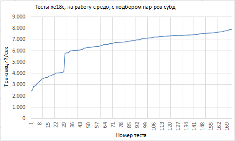
In the form of a graph, if the tests are ordered by increasing metric values, the picture looks like this:
Some data corresponding to the extreme values of the metric:

Here, in the screenshot of the results, let me clarify: the values of the tuning vector are given in the terms of the fitness function code, not in terms of the number-list of parameters/ranges of parameter values formulated earlier in the text.
Well. Whether this is a lot or a little, ~8k tps: that is a separate question.
In the context of the laboratory work, this figure is not crucial, the dynamics of how this value changes is what matters.
The dynamics here are good.
It is clear that, at the very least, one factor significantly influencing the metric value is covered by the GA algorithm as it iterates over the vector chromosomes.
Given the quite lively dynamics of the values of the curve, there is at least one more factor that, although significantly smaller, still has an impact.
Here we need attribute-importance analysis to understand which attributes (in this case, components of the tuning vector) and how strongly influence the metric value.
From this information, we can understand which factors were affected by the changes in significant attributes.
Execute attribute-importance in various ways.
For these purposes, I like the algorithm randomForest of the same name R package (as I understand its operation in general and its approach to assessing the importance of attributes in particular, it builds a model of the response variable's dependence on the attributes.)
randomForestIn our case, the response variable is the metric obtained from the database in load tests:
tps And the attributes are the components of the tuning vector.;
So, it
evaluates the importance of each attribute in the model with two numbers: randomForest %IncMSE — how the presence/absence of this attribute in the model changes the MSE quality of this model (Mean Squared Error); And IncNodePurity — this number reflects how effectively the dataset with observations can be divided based on this attribute's values, such that one part contains data with one value of the explained metric, and the other part contains another value of the metric.
So, that is: how much of a classifying attribute this is (the clearest explanation about random forest I've seen in Russian)
Working-R-class code for processing the dataset with the results of load tests: ).
x=NULL v_data_file=paste('tmp/data1.dat',sep="") x=read.table(v_data_file, header = TRUE, sep = ";", dec=",", quote = ""'", stringsAsFactors=FALSE) colnames(x)=c('metric','rgsize','rgcount','lamp','cmtl','cmtw','lgbffr','lct','dbwrp','undo_retention','tprs','disk_async_io','filesystemio_options','db_block_checking','db_block_checksum')idxTrain=sample(nrow(x),as.integer(nrow(x)*0.7)) idxNotTrain=which(! 1:nrow(x) %in% idxTrain ) TrainDS=x[idxTrain,] ValidateDS=x[idxNotTrain,]library(randomForest) #mtry=as.integer( sqrt(dim(x)[2]-1) ) rf=randomForest(metric ~ ., data=TrainDS, ntree=40, mtry=3, replace=T, nodesize=2, importance=T, do.trace=10, localImp=F) ValidateDS$predicted=predict(rf, newdata=ValidateDS[,colnames(ValidateDS)!="metric"], type="response") sum((ValidateDS$metric-ValidateDS$predicted)^2) rf$importance
You can manually tune the algorithm's hyperparameters and, based on the model's quality, choose a more accurate model for predictions on the validation dataset.You can write a function for this work (by the way, again, based on some optimization algorithm).
You can use the R package
caret caret, it doesn’t matter.
As a result, in this case, we arrive at the following outcome to evaluate the importance of the attributes:
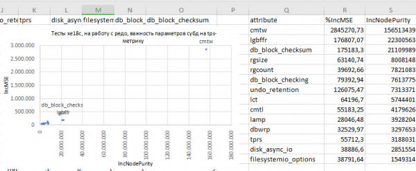
So, we can proceed to the global considerations:
- It turns out that the most significant parameter in these testing conditions was
commit_wait
Technically, it defines the mode for executing io operations for writing redo data from the log buffer of the database to the current log group: synchronous or asynchronous.
Valuenowaitwhich results in a nearly vertical, multiple increase in the tps-metric value: this is the inclusion of async io mode in redo groups.
A separate question is whether or not this should be done in a production database. Here, I limit myself to stating: this is a significant factor. - It logically follows that the size of the log buffer of the database turns out to be a significant factor.
The smaller the size of the log buffer, the lower its buffering capacity, leading to more frequent overflows and/or an inability to allocate free space for a new batch of redo data.
Thus, there are delays associated with the allocation of space in the log buffer and/or the flushing of redo data from it to the redo groups.
These delays, of course, should and do impact the database's transaction throughput. - Parameter
db_block_checksum: well, that’s also generally clear — transaction processing leads to the formation of dirty blocks in the database's buffer cache.
Which, with checksum validation of the data blocks enabled, the database has to process — calculate these checksums from the data block body and compare them with what is written in the data block header: matches / does not match.
Such work cannot help but delay data processing, and accordingly, the parameter and the mechanism that defines this parameter become significant.
That’s why the vendor offers several values for this parameter in the documentation and notes that yes, there will be an impact, but here are the different values, including 'off', and the varied impacts, from which you can choose.
And the overall conclusion.
The approach turns out to be quite effective.
It quite well allows, in the early stages of load testing a certain service system, to select its optimal configuration under load without delving too deeply into the intricacies of system tuning.
However, it does not completely exclude the need for understanding: one must know about the 'controls' and the permissible ranges of rotation of these controls.
Subsequently, this approach can quickly find the optimal configuration of the system.
And based on the testing results, one can obtain information about the nature of the relationship between quality metrics of the system's performance and the values of its tuning parameters.
This, of course, should contribute to the development of a deeper understanding of the system and its functioning, at least under the given load.
Practically, this means weighing the costs of understanding the configurable system against the expenses for preparing such performance testing.
I would like to emphasize that in this approach, the adequacy of the system testing to the conditions it will face in production usage is critically important.
Thank you for your attention and time.
Source: habr.com
