Cheat sheet for quick Data preprocessing

Often, people entering the field of Data Science have unrealistic expectations of what lies ahead. Many believe they will effortlessly write neural networks, create a voice assistant like Iron Man, or outsmart everyone in financial markets.
But the work Data of a Scientist is data-driven, and one of the most crucial and time-consuming aspects is processing the data before feeding it into a neural network or analyzing it in a specific way.

In this article, our team will outline how to easily and quickly process data with a step-by-step guide and code. We've aimed to make the code versatile enough to be applicable to different datasets.

Many professionals may not find anything extraordinary in this article, but beginners could gain new insights, and anyone who has longed to create a separate notebook for quick and structured data processing can copy the code and modify it to their needs, or download a ready-made notebook from GitHub.

You've received a dataset. What’s next?

So, the standard: you need to understand what you are dealing with, the overall picture. For this, we use pandas to simply identify different data types.

import pandas as pd #importing pandas
import numpy as np  #importing numpy
df = pd.read_csv("AB_NYC_2019.csv") #reading the dataset and storing it in df variable

df.head(3) #looking at the first 3 rows to understand how the values appear

df.info() #Displaying information about the columns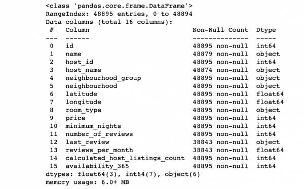

Let's look at the values in the columns:

1. Does the number of rows in each column match the overall row count?
2. What is the essence of the data in each column?
3. Which column do we want to make the target for predictions?

Answers to these questions will allow us to analyze the dataset and sketch a plan for the immediate actions.

Also, for a deeper look at the values in each column, we can use the pandas describe() function. However, a drawback of this function is that it does not provide information about columns with string values. We will address those later.

df.describe()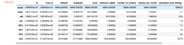

The Magic of Visualization

Let’s look at where we have missing values at all:

import seaborn as sns
sns.heatmap(df.isnull(),yticklabels=False,cbar=False,cmap='viridis')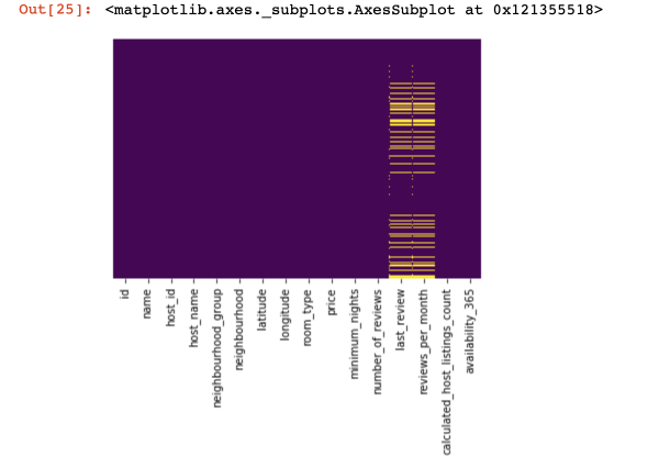

That was a brief overview; now, we will get into more interesting things.

Let's try to find and, if possible, remove the columns that contain only one unique value across all rows (they will not affect the result):

df = df[[c for c
        in list(df)
        if len(df[c].unique()) > 1]] #Overwrite the dataset, keeping only those columns with more than one unique value

Now we protect ourselves and the success of our project from duplicate rows (rows containing the same information in the same order as any existing row):

df.drop_duplicates(inplace=True) #We do this if we consider it necessary.
                                 #In some projects, removing such data from the start may not be advisable.

We divide the dataset into two: one with qualitative values and another with quantitative values

Here, we need to make a small clarification: if the rows with missing data for qualitative and quantitative data do not correlate significantly with each other, we will need to decide what to sacrifice — all rows with missing data, only part of them, or specific columns. If the rows do correlate, we have every right to split the dataset into two. Otherwise, we will first need to address the rows where missing data in qualitative and quantitative data do not correlate, and only then divide the dataset.

df_numerical = df.select_dtypes(include = [np.number])
df_categorical = df.select_dtypes(exclude = [np.number])

We do this to make it easier for us to process these two different types of data — later we will understand how much this simplifies our lives.

Working with quantitative data

The first thing we should do is determine if there are any ‘spy columns’ in the quantitative data. We call these columns so because they masquerade as quantitative data but actually operate as qualitative.

How can we identify them? Of course, it all depends on the nature of the data you are analyzing, but generally, such columns may have few unique data points (around 3-10 unique values).

print(df_numerical.nunique())

Once we identify the spy columns, we will move them from quantitative data to qualitative:

spy_columns = df_numerical[['column1', 'column2', 'column3']]#extracting spy columns and saving to a separate dataframe
df_numerical.drop(labels=['column1', 'column2', 'column3'], axis=1, inplace = True)#removing these columns from numerical data
df_categorical.insert(1, 'column1', spy_columns['column1']) #adding the first spy column to categorical data
df_categorical.insert(1, 'column2', spy_columns['column2']) #adding the second spy column to categorical data
df_categorical.insert(1, 'column3', spy_columns['column3']) #adding the third spy column to categorical data

Finally, we have completely separated numerical data from categorical data and we can now work with them properly. First, we need to understand where we have missing values (NaN, and in some cases, 0 will be considered as missing values).

for i in df_numerical.columns:
    print(i, df[i][df[i]==0].count())

At this stage, it is important to understand in which columns zeroes may indicate missing values: is it related to how the data was collected? Or could it be related to the values themselves? These questions need to be answered on a case-by-case basis.

So, if we have decided that data may be missing where there are zeroes, we should replace zeroes with NaN to make it easier to work with these lost data later:

df_numerical[["column 1", "column 2"]] = df_numerical[["column 1", "column 2"]].replace(0, nan)

Now let's see where we have missing data:

sns.heatmap(df_numerical.isnull(), yticklabels=False, cbar=False, cmap='viridis') # We can also use df_numerical.info()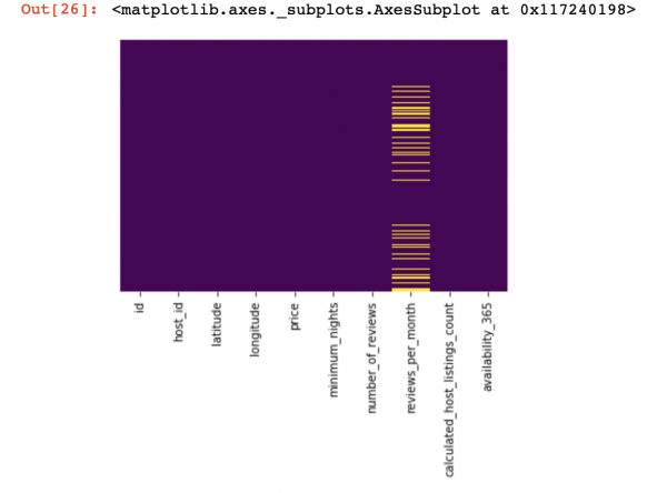

Here, the values in the columns that are missing should be highlighted in yellow. And the most interesting part begins now — how to deal with these values? Should we delete rows with these values or columns? Or should we fill these empty values with something else?

Here is an approximate scheme that may help you figure out what can be done with missing values:

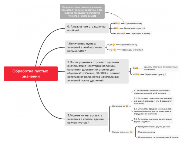
0. Remove unnecessary columns

df_numerical.drop(labels=["column1", "column2"], axis=1, inplace=True)

1. Is the number of missing values in this column greater than 50%?

print(df_numerical.isnull().sum() / df_numerical.shape[0] * 100)

df_numerical.drop(labels=["column1", "column2"], axis=1, inplace=True)#Removing if any column has more than 50 missing values

2. Remove rows with missing values

df_numerical.dropna(inplace=True) #Removing rows with empty values if there is enough data left for training

3.1. Inserting a random value

import random #importing random
df_numerical["column"].fillna(lambda x: random.choice(df[df[column] != np.nan]["column"]), inplace=True) #inserting random values into empty cells in the table

3.2. Inserting a constant value

from sklearn.impute import SimpleImputer #importing SimpleImputer to help insert values
imputer = SimpleImputer(strategy='constant', fill_value="") #inserting a specific value using SimpleImputer
df_numerical[["new_column1", 'new_column2', 'new_column3']] = imputer.fit_transform(df_numerical[['column1', 'column2', 'column3']]) #Applying this to our table
df_numerical.drop(labels=["column1", "column2", "column3"], axis=1, inplace=True) #Removing columns with old values

3.3. Inserting the mean or most frequent value

from sklearn.impute import SimpleImputer #importing SimpleImputer to help insert values
imputer = SimpleImputer(strategy='mean', missing_values=np.nan) #instead of mean, most_frequent can also be used
df_numerical[["new_column1", 'new_column2', 'new_column3']] = imputer.fit_transform(df_numerical[['column1', 'column2', 'column3']]) #Applying this to our table
df_numerical.drop(labels=["column1", "column2", "column3"], axis=1, inplace=True) #Removing columns with old values

3.4. Inserting a value computed by another model

Sometimes values can be computed using regression models, utilizing models from the sklearn library or other similar libraries. Our team will dedicate a separate article on how this can be done in the near future.

So, for now, the narrative on quantitative data will pause, as there are many other nuances on how to better conduct data preparation and preprocessing for different tasks. The foundational aspects for quantitative data have been covered in this article, and now it's time to return to qualitative data, which we separated a few steps back from quantitative data. You can modify this notebook as you wish, tailoring it for various tasks to make data preprocessing very quick!

Qualitative data

The One-hot encoding method is primarily used for categorical data to format it from string (or object) to numeric. Before we move on to this point, let's use the diagram and code above to understand missing values.

df_categorical.nunique()

sns.heatmap(df_categorical.isnull(), yticklabels=False, cbar=False, cmap='viridis')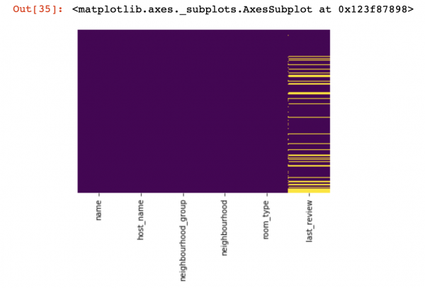

0. Remove unnecessary columns

df_categorical.drop(labels=["column1", "column2"], axis=1, inplace=True)

1. Is the number of missing values in this column greater than 50%?

print(df_categorical.isnull().sum() / df_numerical.shape[0] * 100)

df_categorical.drop(labels=["column1", "column2"], axis=1, inplace=True) # Remove if any column has more than 50% missing values

2. Remove rows with missing values

df_categorical.dropna(inplace=True) # Remove rows with missing values if enough data remains for training

3.1. Inserting a random value

import random
df_categorical["column"].fillna(lambda x: random.choice(df[df[column] != np.nan]["column"]), inplace=True)

3.2. Inserting a constant value

from sklearn.impute import SimpleImputer
imputer = SimpleImputer(strategy='constant', fill_value="")
df_categorical[["new_column1", 'new_column2', 'new_column3']] = imputer.fit_transform(df_categorical[['column1', 'column2', 'column3']])
df_categorical.drop(labels=["column1", "column2", "column3"], axis=1, inplace=True)

So, we finally dealt with missing values in categorical data. Now it's time to perform one-hot encoding for the values in your database. This method is commonly used so that your algorithm can learn from categorical data.

def encode_and_bind(original_dataframe, feature_to_encode):
    dummies = pd.get_dummies(original_dataframe[[feature_to_encode]])
    res = pd.concat([original_dataframe, dummies], axis=1)
    res = res.drop([feature_to_encode], axis=1)
    return(res)

features_to_encode = ["column1", "column2", "column3"]
for feature in features_to_encode:
    df_categorical = encode_and_bind(df_categorical, feature)

So, we finally finished processing categorical and numerical data separately — it's time to combine them back.

new_df = pd.concat([df_numerical, df_categorical], axis=1)

After merging the datasets into one, we can use data transformation with MinMaxScaler from the sklearn library. This will scale our values between 0 and 1, which will aid in training the model in the future.

from sklearn.preprocessing import MinMaxScaler
min_max_scaler = MinMaxScaler()
new_df = min_max_scaler.fit_transform(new_df)

This data is now ready for everything — neural networks, standard ML algorithms, etc!

In this article, we did not consider working with data related to time series, as slightly different techniques for processing such data should be used depending on your task. In the future, our team will dedicate a separate article to this topic, and we hope it will bring something interesting, new, and useful into your life, just like this one.

Source: habr.com