🥇Using AI for extreme image compression

Data-driven algorithms, such as neural networks, have taken the world by storm. Their development is driven by several factors, including affordable and powerful hardware and vast amounts of data. Neural networks are currently at the forefront of all things related to "cognitive" tasks, such as image recognition, natural language understanding, etc. However, they should not be limited to these tasks. This material discusses a method for image compression using neural networks through residual learning. The approach presented in the article performs faster and better than standard codecs. Diagrams, equations, and, of course, a table with tests are available in the article.

This article is based on this work. It is assumed that you are familiar with neural networks and their concepts convolution and loss function.

What is image compression, and what types are there?

Image compression is the process of converting an image in such a way that it takes up less space. Simply storing images would take up a lot of space; therefore, codecs such as JPEG and PNG exist to reduce the size of the original image.

As is known, there are two types of image compression: lossless and lossy. As the names suggest, lossless compression allows for the recovery of the original image data, while lossy compression loses some data during the compression process. For example, JPG is a lossy algorithm [note for the translator — primarily, let’s also not forget about lossless JPEG], while PNG is a lossless algorithm.

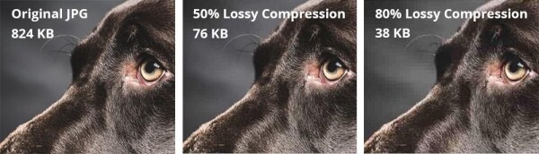
Comparison of lossless and lossy compression

Note that the image on the right has many block artifacts. This is lost information. Neighboring pixels of similar colors are compressed as one area to save space, but this results in the loss of data about the actual pixels. Of course, the algorithms used in codecs like JPEG, PNG, etc., are much more complex, but this is a good intuitive example of lossy compression. Lossless compression is good, but lossless compressed files take up a lot of disk space. There are more efficient ways to compress images without losing a significant amount of information, but they are quite slow, and many use iterative approaches. This means they cannot be run in parallel on multiple CPU or GPU cores. Such a limitation makes them entirely impractical for everyday use.

Input of a convolutional neural network

If something needs to be calculated and the calculations can be approximate, add a neural network. The authors used a fairly standard convolutional neural network to enhance image compression. The proposed method not only performs on par with the best solutions (if not better), it also supports parallel computing, resulting in a significant speed increase. The reason is that convolutional neural networks (CNN) are very good at extracting spatial information from images, which is then represented in a more compact form (for instance, only the 'important' bits of the image are stored). The authors aimed to leverage this capability of CNNs to better represent images.

Architecture

The authors proposed a dual network. The first network takes an image as input and generates a compact representation (ComCNN). The output of this network is then processed by a standard codec (e.g., JPEG). After processing by the codec, the image is passed to the second network, which 'fixes' the image from the codec in an attempt to restore the original image. The authors named this network the reconstructing CNN (RecCNN). Similar to GAN, both networks are trained iteratively.

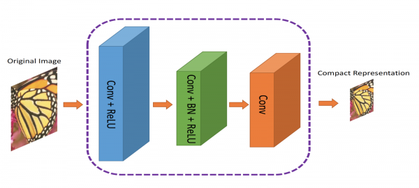
ComCNN The compact representation is sent to the standard codec

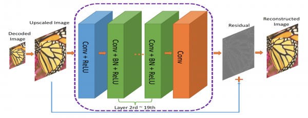
RecCNN. The output of ComCNN is upscaled and sent to RecCNN, which will attempt to learn the remainder

The codec output scales with increase and is then passed to RecCNN. RecCNN will attempt to output an image that resembles the original as closely as possible.

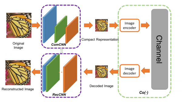
A framework for image compression. Co(.) is an image compression algorithm. The authors applied JPEG, JPEG2000, and BPG.

What is a residual?

Residual can be seen as a post-processing step to 'enhance' the image decoded by the codec. Having a larger amount of 'information' about the world, the neural network can make cognitive decisions about what to correct. This idea is based on residual learning, details of which you can read about here.

Loss functions

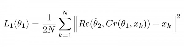
Two loss functions are used because we have two neural networks. The first, ComCNN, is labeled as L1 and is defined as follows:

Loss function for ComCNN

Explanation

This equation might seem complex, but it is actually a standard (mean squared error) formula. MSE. ||² denotes the norm of the vector that they contain.

Equation 1.1

Cr denotes the output of ComCNN. θ denotes the learnable parameters of ComCNN, XK is the input image.

Equation 1.2

Re() denotes RecCNN. This equation simply passes the value of equation 1.1 to RecCNN. θ denotes the learnable parameters of RecCNN (the hat on top indicates that the parameters are fixed).

Intuitive definition

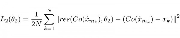
Equation 1.0 will cause ComCNN to adjust its weights in such a way that after reconstruction with RecCNN, the final image looks as close as possible to the input image. The second loss function for RecCNN is defined as follows:

Equation 2.0

Explanation

Again, the function may seem complicated, but this is mostly a standard loss function for neural networks (MSE).

Equation 2.1

Co() denotes the codec output, x with a hat on top signifies the output of ComCNN. θ2 are the learnable parameters of RecCNN. res() simply represents the residual output of RecCNN. It's worth noting that RecCNN is trained on the difference between Co() and the input image, but not on the input image itself.

Intuitive definition

Equation 2.0 will cause RecCNN to adjust its weights so that the output looks as similar as possible to the input image.

Training Scheme

Models are trained iteratively, similar to GANThe weights of the first model are fixed while the weights of the second model are updated, then the weights of the second model are fixed while the first model is trained.

Tests

The authors compared their method with existing methods, including simple codecs. Their method performs better than others while maintaining high speed on the appropriate hardware. Additionally, the authors attempted to use only one of the two networks and noted a drop in performance.

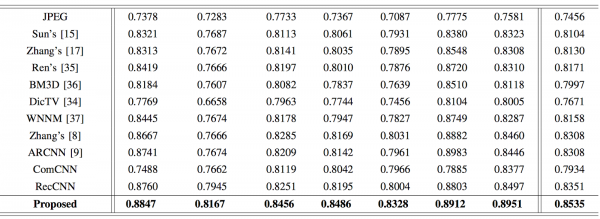
Comparison of the Structural Similarity Index (SSIM). Higher values indicate better similarity to the original. The authors' results are highlighted in bold.

Conclusion

We explored a new way to apply deep learning for image compression, discussing the potential use of neural networks for tasks beyond the 'common' ones, such as image classification and natural language processing. This method not only meets modern requirements but also allows for much faster image processing.

Studying neural networks has become easier, as we have created a promo code specifically for Habr readers. HABR, providing an additional 10% discount on the discount indicated on the banner.