

Introduction
 "You have to run at full speed just to stay in place,
and if you want to get somewhere, you have to run at least twice as fast!"
(c) Alice in Wonderland
Some time ago, I was asked to give a lecture to the analysts of our company on the topic of data model design. Since we often spend long periods on projects (sometimes for several years), we tend to overlook developments in the IT technology landscape. In our company, (as it turns out), NoSQL databases are not used in many projects (at least not yet), so in my lecture, I focused particularly on them using HBase as an example and aimed to tailor the material for those who have never worked with them. Specifically, I illustrated some aspects of data model design based on an example I read a few years ago While examining examples, I compared several approaches to the same problem to better convey the main ideas to the audience.
Recently, "out of boredom," I wondered (the long May holidays during quarantine especially encourage this) how much the theoretical findings align with real practice? Thus, the idea for this article was born. A developer who has been working with NoSQL for some time might not gain anything new from it (and might therefore skip half the article). But for analysts, who haven't worked closely with NoSQL yet, I believe this will be useful for gaining a basic understanding of the features of data model design for HBase.
Example Review
In my opinion, before starting to use NoSQL databases, it is important to carefully consider the pros and cons. Often, the task can likely be solved with traditional relational DBMS. Therefore, it is better not to use NoSQL without substantial reasons. If the decision to utilize a NoSQL database has been made, it should be taken into account that the design approaches are somewhat different here. In particular, some of them may be unfamiliar to those who have only dealt with relational DBMS before (based on my observations). In the 'relational' world, we typically start from domain modeling and then perform model denormalization if necessary. In NoSQL, however, we must immediately consider the expected data usage scenarios and initially denormalize the data. Additionally, there are several other differences that will be discussed below.
Let's consider the following 'synthetic' problem, which we will continue to work on:
We need to design a structure to store a list of friends for users of some abstract social network. For simplicity, we will assume that all relationships are directed (like on Instagram, not LinkedIn). The structure should allow us to effectively:
- Answer the question of whether user A reads user B (reading pattern)
- Allow adding/removing relationships when user A subscribes/unsubscribes from user B (data modification pattern)
Of course, there are many ways to solve the problem. In a regular relational database, we would likely just create a relationship table (possibly with types if, for example, we need to store the user group: family, work, etc., that includes this 'friend'), and to optimize access speed, we would add indexes/partitioning. Most likely, the final table would look something like this:
user_id
friend_id
Vasya
Petya
Vasya
Olya
For clarity and better understanding, I will indicate names instead of IDs here and below
In the case of HBase, we know that:
- effective searching that does not lead to a full table scan is possible exclusively by key
- That's why writing familiar SQL queries to such databases is a bad idea; technically, you could send an SQL query with Joins and other logic from Impala to HBase, but how effective would that be...
Therefore, we have to use the user ID as a key. The first thought on how and where to store the IDs of friends could be the idea of storing them in columns. This most obvious and 'naive' option would look something like this (let's call it Option 1 (default), for future reference):
RowKey
Columns
Vasya
1: Petya
2: Olya
3: Dasha
Petya
1: Masha
2: Vasya
Here, each row corresponds to one user of the network. The columns have names: 1, 2, … — which correspond to the number of friends, and the IDs of friends are stored in these columns. It’s important to note that each row will have a different number of columns. In the example above, one row has three columns (1, 2, and 3), while the other has only two (1 and 2) – here we have utilized two properties of HBase that are not present in relational databases:
- the ability to dynamically change the composition of columns (add a friend -> add a column, remove a friend -> remove a column)
- the different rows can have varying sets of columns
Let's check our structure against the task requirements:
- Data reading: to determine if Vasya is following Olya, we will need to read the entire row by RowKey = 'Vasya' and iterate through the column values until we 'find' Olya in them. Alternatively, we can iterate through all column values, 'not find' Olya, and return False;
- Data modification: adding a friend: for such a task, we will also need to read the entire row by RowKey = 'Vasya' to count his total number of friends. This total number of friends is necessary for us to determine the column number where we need to write the ID of the new friend.
- Data modification: removing a friend:
- We need to read the entire row by RowKey = 'Vasya' and iterate through columns to find the one that contains the ID of the friend to be removed;
- Next, after deleting a friend, we need to 'shift' all data by one column to avoid 'gaps' in their numbering.
Now, let's evaluate how efficient the algorithms we need to implement on the 'hypothetical application' side will be, using Let's denote the size of our hypothetical social network as n. Then the maximum number of friends for one user can be (n-1). We can disregard this (-1) for our purposes, as it is insignificant within the context of O-notation.
- Data reading: it is necessary to read the entire row and check all its columns in the limit. Thus, the upper estimate of costs will be approximately O(n)
- Data modification: adding a friend: to determine the number of friends, it is necessary to check all the columns of the row, after which a new column will be added => O(n)
- Data modification: removing a friend:
- Similarly to adding – it is necessary to check all columns in the limit => O(n)
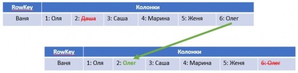
- After removing columns, we need to 'shift' them. If we implement this 'directly', it will require up to (n-1) operations in the limit. However, we will apply a different approach in the practical part, which will achieve a 'pseudo-shift' in a fixed number of operations – that is, it will take constant time regardless of n. This constant time (specifically, O(2)) can be ignored compared to O(n). The approach is illustrated in the figure below: we simply copy data from the 'last' column to the one from which we need to delete data, and then we delete the last column:

In total, in all scenarios, we have achieved an asymptotic computational complexity of O(n).
You may have already noticed that we almost always have to read the entire row from the database, and in two out of three cases, just to check all columns and count the total number of friends. Therefore, as an optimization attempt, we can add a 'count' column that stores the total number of friends for each user in the network. In this case, we don't have to read the entire row to count the total number of friends; we can read just one 'count' column. The main thing is to remember to update 'count' when manipulating data. Thus, we obtain an improved Option 2 (count):
RowKey
Columns
Vasya
1: Petya
2: Olya
3: Dasha
count: 3
Petya
1: Masha
2: Vasya
count: 2
Compared to the first option:
- Data reading: to answer the question 'Does Vasya read Olya?' nothing has changed => O(n)
- Data modification: adding a friend: We have simplified the addition of a new friend, as we no longer need to read the entire row and go through its columns; instead, we can get the value of the 'count' column and thus immediately determine the column number for inserting a new friend. This reduces the computational complexity to O(1).
- Data modification: removing a friend: When removing a friend, we can also utilize this column to reduce the number of input-output operations when 'shifting' data one cell to the left. However, the need to iterate through columns to find the one that needs to be deleted still remains, hence => O(n).
- On the other hand, now we must update the 'count' column every time we update the data, but this takes constant time, which can be neglected within the bounds of O-notation.
Overall, option 2 seems slightly more optimal, but it is more of an 'evolution rather than a revolution'. To make a 'revolution', we will need Option 3 (col).
Let's turn everything 'upside down': we will assign the column name as the user identifier.! What will be recorded in that column is no longer important to us; it can simply be the number 1 (generally, one could store something useful there, like a group 'family/friends/etc.'). This approach might surprise an unprepared 'layman' who has had no prior experience with NoSQL databases, but it allows us to leverage HBase's potential in this task much more effectively:
RowKey
Columns
Vasya
Petya: 1
Olya: 1
Dasha: 1
Petya
Masha: 1
Vasya: 1
Here, we gain several advantages right away. To understand them, let's analyze the new structure and evaluate the computational complexity:
- Data reading: to answer the question of whether Vasya is subscribed to Olya, it is enough to read one column 'Olya': if it exists, the answer is True; if not, it is False => O(1).
- Data modification: adding a friend: Adding a friend: it is enough to simply add a new column 'friend ID' => O(1).
- Data modification: removing a friend: it is enough to simply delete the column 'friend ID' => O(1).
As we can see, a significant advantage of this storage model is that in all the necessary scenarios, we operate with only one column, avoiding reading the entire row from the database and, moreover, iterating through all columns of that row. One could stop here, but…
One can ponder and go a bit further down the path of performance optimization and reducing I/O operations when accessing the database. What if we store the complete relationship information directly in the string key? That is, make the key composite, like userID.friendID? In this case, we may not even need to read the row's columns at all.Option 4 (row)):
RowKey
Columns
Vasya.Petya
Petya: 1
Vasya.Olya
Olya: 1
Vasya.Dasha
Dasha: 1
Petya.Masha
Masha: 1
Petya.Vasya
Vasya: 1
It is evident that the evaluation of all scenarios for data manipulation in this structure, just like in the previous option, will also be O(1). The difference from option 3 will be exclusively in the efficiency of I/O operations in the database.
And the last 'ribbon'. It's easy to notice that in option 4 our row key will have variable length, which may affect performance (let's remember that HBase stores data as a set of bytes and rows in tables are sorted by key). Plus, we have a delimiter that may need to be processed in some scenarios. To eliminate this impact, one could use hashes of userID and friendID, and since both hashes will have a fixed length, they can simply be concatenated without a delimiter. Then the data in the table would look like this.Option 5 (hash)):
RowKey
Columns
dc084ef00e94aef49be885f9b01f51c01918fa783851db0dc1f72f83d33a5994
Petya: 1
dc084ef00e94aef49be885f9b01f51c0f06b7714b5ba522c3cf51328b66fe28a
Olya: 1
dc084ef00e94aef49be885f9b01f51c00d2c2e5d69df6b238754f650d56c896a
Dasha: 1
1918fa783851db0dc1f72f83d33a59949ee3309645bd2c0775899fca14f311e1
Masha: 1
1918fa783851db0dc1f72f83d33a5994dc084ef00e94aef49be885f9b01f51c0
Vasya: 1
It is apparent that the algorithmic complexity when working with such a structure in the scenarios we are considering will be the same as in option 4 – that is, O(1).
In summary, let's consolidate all our computational complexity assessments into one table:
Adding a friend
Checking a friend
Removing a friend
Option 1 (default)
O(n)
O(n)
O(n)
Option 2 (count)
O(1)
O(n)
O(n)
Option 3 (column)
O(1)
O(1)
O(1)
Option 4 (row)
O(1)
O(1)
O(1)
Option 5 (hash)
O(1)
O(1)
O(1)
As can be seen, options 3-5 appear to be the most preferable and theoretically ensure the execution of all necessary data manipulation scenarios in constant time. In our task's condition, there is no explicit requirement to obtain a list of all friends of the user, but in real project activities, it would be wise for us as good analysts to 'foresee' that such a task may arise and 'prepare for it'. Thus, my preference leans toward option 3. However, it is quite possible that in a real project, this request could have already been addressed by other means, so without a comprehensive view of the entire task, it is better not to draw final conclusions.
Preparing the experiment
The theoretical considerations outlined above would like to be tested in practice – this was the aim of the idea that emerged during the long weekend. To do this, it is necessary to evaluate the performance of our 'conditional application' across all described usage scenarios of the database, as well as the growth of this time with the increase in the size of the social network (n). The target parameter that interests us and that we will measure during the experiment is the time taken by the 'conditional application' to perform one 'business operation'. By 'business operation', we mean one of the following:
- Adding one new friend
- Checking if user A is a friend of user B
- Removing one friend
Thus, considering the requirements outlined in the original task, the check scenario is shaping up as follows:
- Recording data. Generate a random initial network of size n. To approach the 'real world' more closely, the number of friends for each user is also a random variable. Measure the time it takes for our 'conditional application' to write all the generated data into HBase. Then divide the obtained time by the total number of added friends – this will give us the average time per one 'business operation'.
- Data readingFor each user, compile a list of 'identities' to determine whether the user is subscribed to them or not. The length of the list should be approximately equal to the number of the user's friends, with half of the friends checked returning 'Yes' and the other half returning 'No'. The checks should alternate the responses 'Yes' and 'No', meaning that in every second case, we will have to go through all columns of the row for options 1 and 2. The total check time should then be divided by the number of friends checked to get the average time per subject checked.
- Deleting dataRemove all friends from the user. The order of deletion should be random (i.e., shuffle the original list used for data recording). The total check time should then be divided by the number of friends deleted to get the average time for one check.
The scenarios need to be run for each of the 5 variants of data models and for different sizes of the social network to observe how the time changes as the network grows. Within one n connection in the network, the list of users for checks should naturally be the same for all 5 variants.
For better understanding, I provide below an example of generated data for n=5. The written 'generator' outputs three dictionaries of IDs:
- first – for insertion
- second – for checking
- third – for deletion
{0: [1], 1: [4, 5, 3, 2, 1], 2: [1, 2], 3: [2, 4, 1, 5, 3], 4: [2, 1]} # total 15 friends

{0: [1, 10800], 1: [5, 10800, 2, 10801, 4, 10802], 2: [1, 10800], 3: [3, 10800, 1, 10801, 5, 10802], 4: [2, 10800]} # total 18 subjects checked

{0: [1], 1: [1, 3, 2, 5, 4], 2: [1, 2], 3: [4, 1, 2, 3, 5], 4: [1, 2]} # total 15 friends
As can be seen, all IDs greater than 10,000 in the check dictionary are precisely those that will certainly return False. Insertion, checking, and deletion of 'friends' are performed exactly in the sequence specified in the dictionary.
The experiment was conducted on a laptop running Windows 10, where one Docker container was running the HBase database, and another was running Python with Jupyter Notebook. The Docker setup was allocated 2 CPU cores and 2 GB of RAM. All logic, including the simulation of the 'conditional application' and the 'wrapper' for generating test data and measuring time, was written in Python. The library used for working with HBase was , for calculating hashes (MD5) for variant 5 — hashlib
Taking into account the computing power of the specific laptop, the launch was experimentally chosen for n = 10, 30, … 170 – when the total runtime of the complete test cycle (all scenarios for all variants for all n) was still reasonable and fit within the time of one tea break (approximately 15 minutes).
It should be noted that in this experiment, we are primarily evaluating not the absolute performance figures. Even the relative comparison of the two different variants may not be entirely correct. We are currently interested in the nature of the change in time depending on n, as obtaining time estimates that are 'cleansed' of random and other factors given the aforementioned configuration of the 'test stand' is quite challenging (and this task was not explicitly set).
Experiment results
The first test – how the time taken to populate the friends list changes. The result is shown in the graph below.
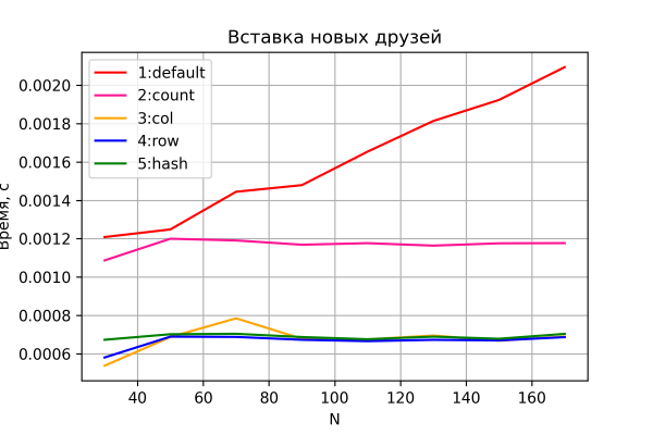
Variants 3-5 predictably show a practically constant time for the 'business operation', which does not depend on the growth of the network size and shows indistinguishable differences in performance.
Variant 2 also shows constant, albeit slightly worse performance, approximately 2 times relative to variants 3-5. This is encouraging, as it aligns with theory – in this variant, the number of input-output operations into/from HBase is exactly twice as high. This may serve as indirect evidence that our test stand provides decent accuracy.
Variant 1 is also predictably the slowest and demonstrates a linear increase in time taken to add a friend based on the size of the network.
Now let's look at the results of the second test.
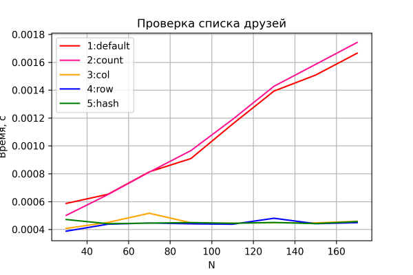
Options 3-5 behave as expected again – constant time, independent of network size. Options 1 and 2 demonstrate linear growth in time as the network size increases, with similar performance. Moreover, option 2 turns out to be slightly slower – apparently due to the need to read and process the additional 'count' column, which becomes more noticeable as n grows. However, I will refrain from any conclusions, as the accuracy of this comparison is relatively low. Additionally, the relations (which option, 1 or 2, is faster) varied from run to run (while maintaining the nature of the dependence and 'running nose to nose').
And the last chart – results of the deletion test.
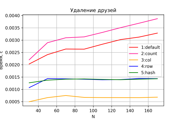
Here again, no surprises. Options 3-5 perform deletions in constant time.
Interestingly, options 4 and 5, unlike the previous scenarios, show slightly worse performance than option 3. Apparently, the operation of deleting a row is more costly than the operation of deleting a column, which is overall logical.
Options 1 and 2, as expected, demonstrate linear growth in time. Moreover, option 2 is consistently slower than option 1 – due to the additional input/output operation for 'maintaining' the count column.
General conclusions of the experiment:
- Options 3-5 demonstrate greater efficiency, as they take advantage of HBase; their performance differs from each other by a constant and is independent of network size.
- The difference between options 4 and 5 was not recorded. But this does not mean that option 5 should not be used. It is quite possible that the experimental scenario, taking into account the specifications of the test stand, did not allow it to be revealed.
- The nature of the time growth required for performing 'business operations' with data generally confirmed the previously obtained theoretical deductions for all options.
Epilogue
The rough experiments conducted should not be taken as absolute truth. There are many factors that were not taken into account and distorted the results (especially noticeable in graphs with a small network size). For instance, the performance of Thrift used by HappyBase, the volume and implementation of the logic I wrote in Python (I can't claim that the code was written optimally and effectively utilized all component capabilities), potential caching features of HBase, background activity of Windows 10 on my laptop, etc. Overall, it can be considered that all theoretical conclusions have been experimentally validated. Or at least, it was not possible to refute them with a 'straightforward attack.'
In conclusion — recommendations for everyone who is just starting to design data models in HBase: detach yourself from previous experience with relational databases and remember the 'commandments':
- When designing, we start from the task and data manipulation patterns, not from the domain model.
- Effective access (without full table scan) – only by key.
- Denormalization.
- Different rows can contain different columns.
- Dynamic column composition.
Source: habr.com
