

Many who are already using — our PostgreSQL plan visualization service, may not be aware of one of its superpowers — transforming a difficult-to-read chunk of server log...
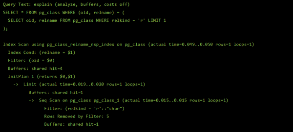
… into a beautifully formatted query with contextual hints about the corresponding nodes in the plan:
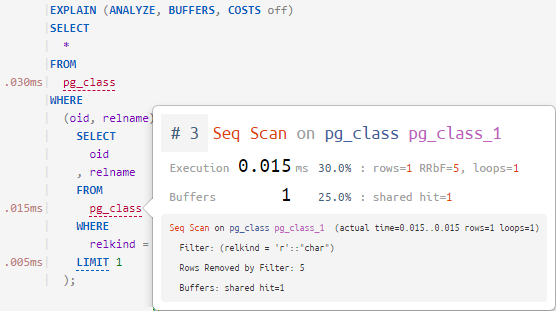
In this decryption of the second part of my I will explain how we managed to do this.
The transcript of the first part, dedicated to typical performance issues and their solutions, can be found in the article .

First, let's tackle the coloring — and we will color not the plan, which we have already beautified, but the query.
We felt that this unformatted ‘sheet’ extracted from the log looks very unattractive and, therefore, inconvenient.
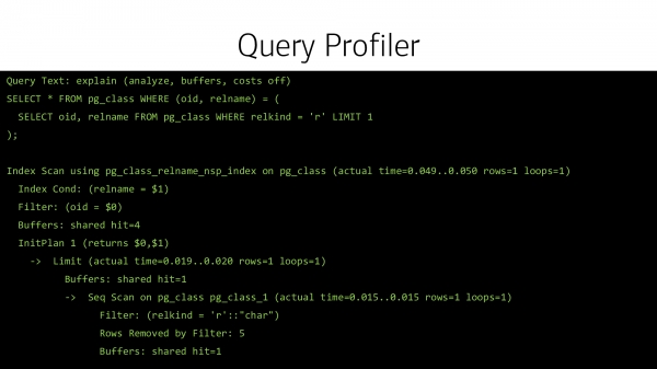
Especially when developers ‘stitch’ the query body in a single line in the code (this is, of course, an antipattern, but it happens). Yikes!
Let's illustrate this more beautifully.
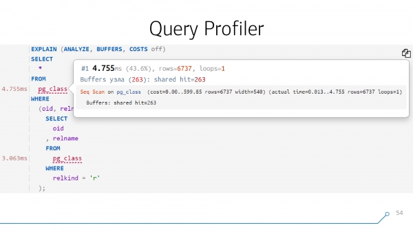
If we can draw it nicely, meaning analyze and reconstruct the query body, we can then ‘attach’ hints to each object of that query — explaining what happened at the corresponding point in the plan.
The query syntax tree
To do this, the query needs to be parsed first.
Since our , we created a small module for it, you can . In fact, this serves as extended ‘bindings’ to the internals of the PostgreSQL parser itself. So, it’s just a binary compiled grammar with bindings from the NodeJS side. We based this on existing modules — there’s no major secret here.
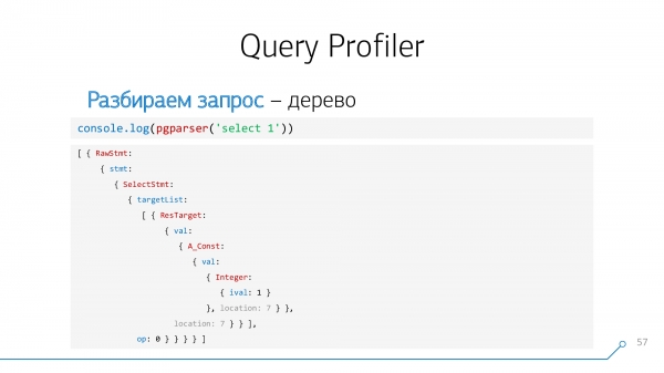
We feed the query body into our function — and get a parsed syntax tree as a JSON object.
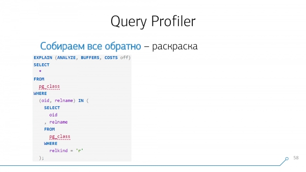
Now we can traverse this tree in reverse to reconstruct the query with the desired indentation, coloring, and formatting. No, this isn’t customizable, but we felt that this would be convenient.
Mapping query nodes to the plan
Now let's see how we can combine the plan we parsed in the first step and the query we parsed in the second.
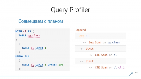
Let's take a simple example — we have a query that forms a CTE and reads from it twice. It generates such a plan.
CTE
If we look closely at it, before version 12 (or starting from it with the keyword MATERIALIZED) the formation .
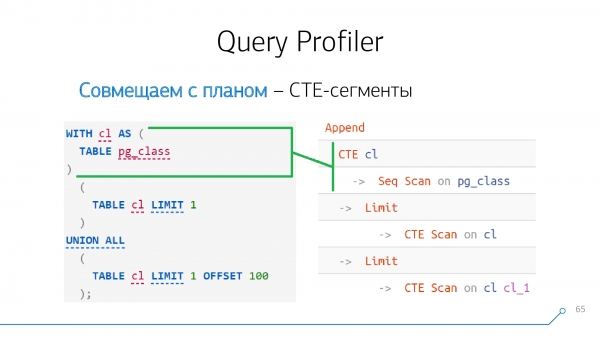
So, if we see in the query the generation of a CTE and somewhere in the plan a node CTE, then these nodes are definitely 'colliding' with each other, we can immediately merge them.
A 'task with a star': CTEs can be nested.
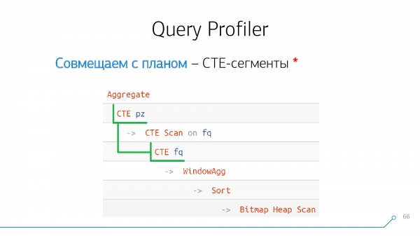
There can be very poorly nested ones, and even ones with the same name. For example, you can create inside CTE A another one CTE X, and at the same level inside CTE B do another one CTE X:
WITH A AS (
  WITH X AS (...)
  SELECT ...
)
, B AS (
  WITH X AS (...)
  SELECT ...
)
...
When matching, you must understand this. Understanding it 'visually' — even seeing the plan, even seeing the body of the query — is very difficult. If your generation of CTE is complex, nested, and the queries are large — then it's almost unconscious.
UNION
If there is a keyword in our query UNION [ALL] (the operator that combines two selections), then in the plan it corresponds to either a node Append, or some Recursive Union.
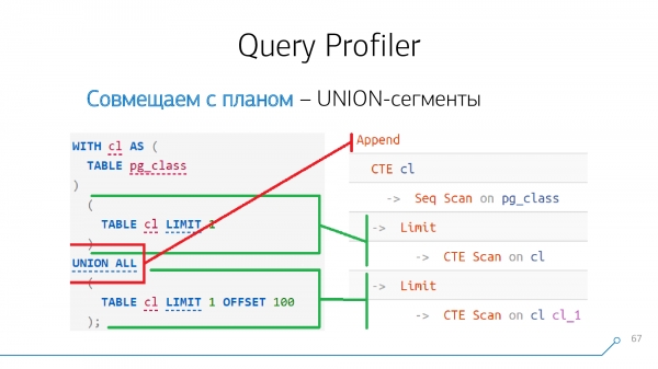
What is 'above' the node UNION is the first child of our node, and what is 'below' is the second. If through UNION several blocks are 'glued' together, then Append- the node will still be only one, but it will have many children according to the order they appear:
  (...) -- #1
UNION ALL
  (...) -- #2
UNION ALL
  (...) -- #3
Append
-> ... #1
-> ... #2
-> ... #3
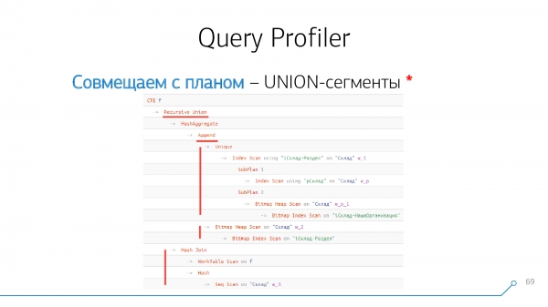
A 'task with a star': inside the generation of a recursive selection (WITH RECURSIVE) there can also be more than one. UNIONBut always recursive is only the very last block after the last UNION. Everything above is one, but another. UNION:
WITH RECURSIVE T AS(
  (...) -- #1
UNION ALL
  (...) -- #2, this ends the generation of the starting state of recursion
UNION ALL
  (...) -- #3, only this block is recursive and can contain references to T
)
...
Such examples must also be 'unpeeled'. In this example, we see that UNION- there were 3 segments in our query. Accordingly, one UNION corresponds to Append- a node, and another one — Recursive Union.
Read-write data
That's it, we've laid it all out, now we know which part of the query corresponds to which part of the plan. And in these parts, we can easily and effortlessly find those objects that are 'read'.
From the point of view of the query, we don't know — is it a table or a CTE, but they are indicated by the same node. RangeVar. In the execution plan, the "readability" aspect is a rather limited set of nodes.
Sequential Scan on [tbl]Bitmap Heap Scan on [tbl]Index [Only] Scan [Backward] using [idx] on [tbl]CTE Scan on [cte]Insert/Update/Delete on [tbl]
We know the structure of the plan and the query, we are aware of the block correspondence, and we know the object names — we make a clear mapping.
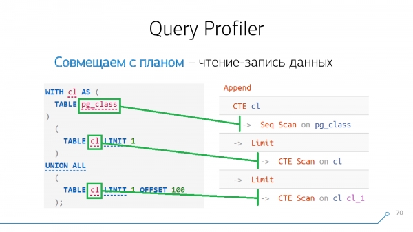
Again, the "starred" task. We take the query, execute it, and we have no aliases — we simply read from the same CTE twice.
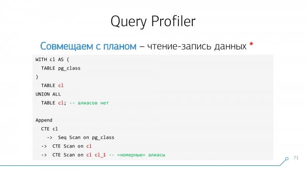
We look at the plan — what's going on? Why did the alias appear? We didn't request it. Where did it come from with such a "number"?
PostgreSQL adds it automatically. We just need to understand that such an alias doesn't make any sense for our purposes of mapping with the plan, it is just added here. Let's not pay attention to it.
The second the "starred" task: if we are reading from a partitioned table, we will get a node Append or Merge Append, which will consist of a large number of "children," each representing some Scanfrom the section table: Sequential Scan, Bitmap Heap Scan or Index Scan. However, in any case, these "children" will not be complex queries — this is how these nodes can be differentiated from Append in UNION.
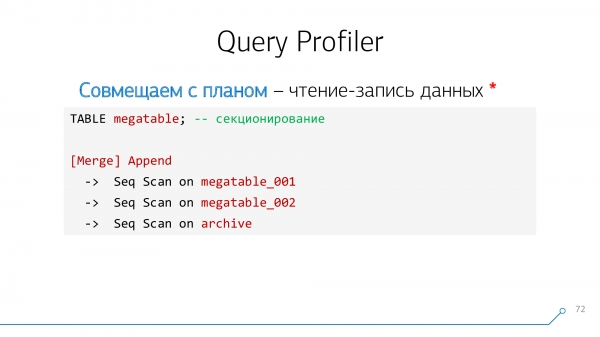
We also understand such nodes, gather them "into one pile", and say: "everything you've read from megatable — it’s here and down the tree".
The "simple" data retrieval nodes
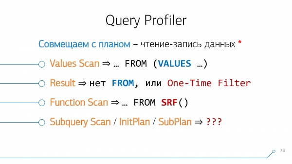
Values Scan in the plan correspond to VALUES in the query.
Result — this is a query without FROM like SELECT 1. Or when you have a known false expression in the WHERE-block (then the attribute arises One-Time Filter):
EXPLAIN ANALYZE
SELECT * FROM pg_class WHERE FALSE; -- or 0 = 1
Result (cost=0.00..0.00 rows=0 width=230) (actual time=0.000..0.000 rows=0 loops=1)
One-Time Filter: false
Function Scan "map" to identically named SRFs.
But with nested queries, it's more complicated — unfortunately, they do not always turn into InitPlan/SubPlan. Sometimes they turn into ... Join or ... Anti Join, especially when you write something like WHERE NOT EXISTS .... And there, combining them does not always work — in the plan's text, there are no corresponding plan nodes for the operators.
Again, the "starred" task: several VALUES in the query. In this case, you will get several nodes in the plan Values Scan.
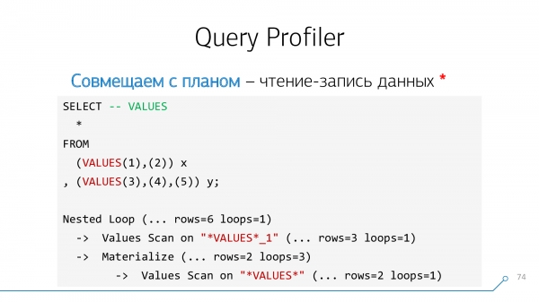
The "numbered" suffixes will help distinguish one from another — it is added precisely in the order of finding the corresponding VALUES-blocks down the query.
Data processing
We seem to have unraveled everything in our query — only left Limit.
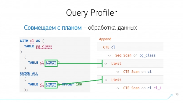
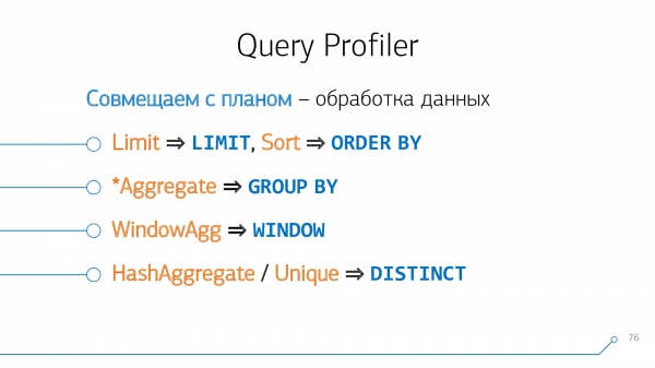
But here everything is simple — such nodes as Limit, Sort, Aggregate, WindowAgg, Unique "map" one-to-one to the corresponding operators in the query, if they exist. There are no "stars" or complications here.
JOIN
Complications arise when we want to combine JOIN with each other. This is not always possible, but it can be done.
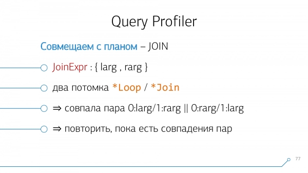
From the perspective of the query parser, we have a node JoinExpr, which has exactly two children — left and right. This is, respectively, what is ‘above’ your JOIN and what is ‘below’ it in the query.
And from the perspective of the plan, this is two children of some * Loop/* Join-node. Nested Loop, Hash Anti Join,… — something like that.
Let's use simple logic: if we have tables A and B that are ‘joining’ with each other in the plan, then in the query they could be arranged either A-JOIN-B, or B-JOIN-A. Let's try combining them this way, and then the other way, and so on until such pairs run out.
Let’s take our syntax tree, take our plan, look at them… doesn’t quite look like it!
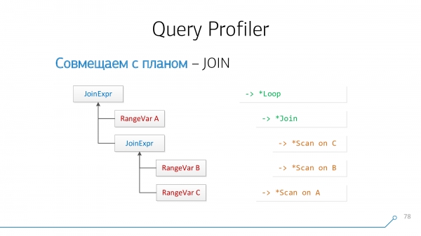
Redrawing it as graphs — oh, it’s starting to look something like something!
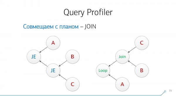
Let’s note that we have nodes that simultaneously have children B and C — we don’t care about the order. Let’s combine them and flip the node picture.
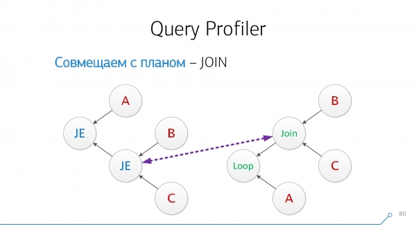
Let’s take another look. Now we have nodes with children A and pairs (B + C) — let’s combine those too.
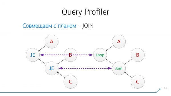
Great! It turns out that we successfully combined these two JOIN from the query with the plan nodes.
Unfortunately, this task is not always solvable.
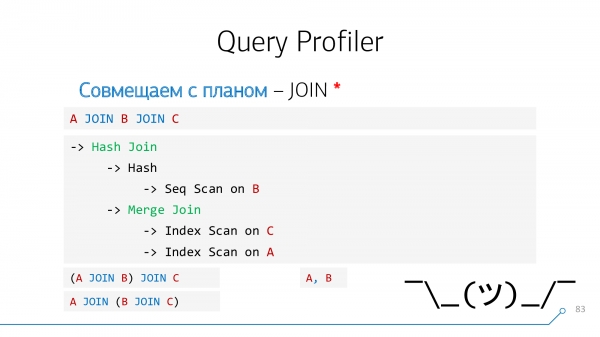
For example, if in the query A JOIN B JOIN C, and in the plan the ‘extreme’ nodes A and C were combined first. And in the query there is no such operator, we have nothing to highlight, nothing to attach the hint to. The same goes for the ‘comma’ when you write A, B.
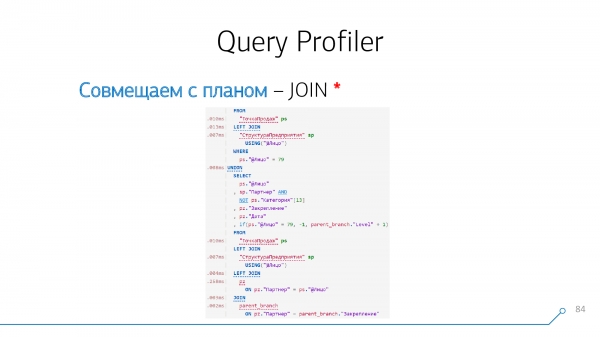
But, in most cases, almost all nodes can be ‘untangled’ and you get a profiling like this on the left by time — literally like in Google Chrome when analyzing your JavaScript code. You see how much time each line and each operator ‘took to execute’.
And to make it easier for you to use all this, we created a storage , where you can save and later find your plans along with associated queries or share the link with someone.
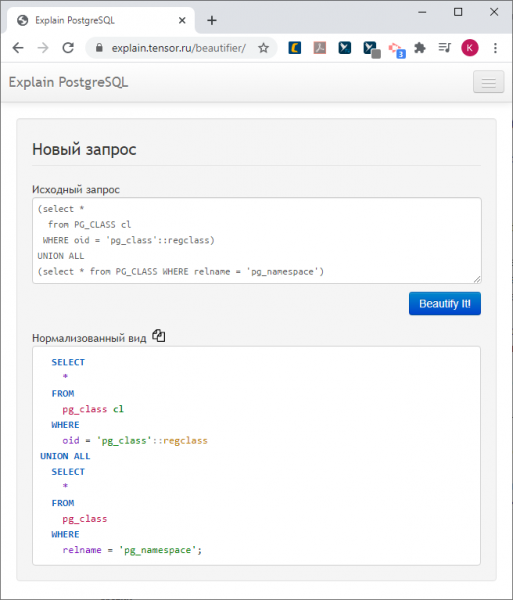
If you just need to put an unreadable query into a reasonable form, use our .
Source: habr.com
