

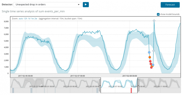
Let's recall that the Elastic Stack is based on the non-relational database Elasticsearch, the web interface Kibana, and data processors (the most famous being Logstash, various Beats, APM, and others). One of the nice additions to this product stack is data analysis using machine learning algorithms. In this article, we will explore what these algorithms are all about. We invite you to read on.
Machine learning is a paid feature of the somewhat free Elastic Stack and is included in the X-Pack package. To start using it, you need to activate a 30-day trial after installation. Once the trial period ends, you can request support for an extension or purchase a subscription. The subscription price is based not on the volume of data but rather on the number of nodes used. While the data volume does influence the number of required nodes, this licensing approach is more budget-friendly for companies. If high performance is not necessary, you can save costs.
ML in the Elastic Stack is written in C++ and operates outside the JVM, in which Elasticsearch itself runs. This means the process (which is called autodetect, by the way) consumes everything that the JVM does not handle. This is not critical on a demo stand, but in a production environment, it's important to allocate separate nodes for ML tasks.
Machine learning algorithms are divided into two categories — and . In the Elastic Stack, the algorithm falls into the 'without a teacher' category. You can refer to to see the mathematical framework of machine learning algorithms.
For conducting analysis, the machine learning algorithm uses data stored in Elasticsearch indices. Jobs for analysis can be created from both the Kibana interface and through the API. If doing this via Kibana, some knowledge of certain things is not strictly necessary. For example, the additional indices that the algorithm uses during its operation.
Additional indices used during the analysis process.ml-state — information about statistical models (analysis settings);
.ml-anomalies-* — results from the operation of the ML algorithms;
.ml-notifications — notification settings based on analysis results.
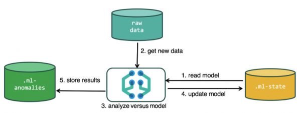
The data structure in an Elasticsearch database consists of indices and the documents stored within them. If we compare this to a relational database, an index can be likened to a database schema, while a document is akin to a record in a table. This comparison is conditional and is provided to simplify understanding of further material for those who have only heard about Elasticsearch.
The same functionality that is available through the web interface is accessible via the API; therefore, for clarity and understanding of the concepts, we will show how to configure it through Kibana. On the left menu, there is a section called Machine Learning, where you can create a new job. In the Kibana interface, this looks like the image below. We will now break down each type of job and demonstrate the types of analysis that can be constructed here.
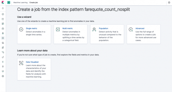
Single Metric — analysis of a single metric, Multi Metric — analysis of two or more metrics. In both cases, each metric is analyzed in isolation, meaning the algorithm does not account for the behavior of concurrently analyzed metrics, as might appear in the case of Multi Metric. To conduct calculations considering the correlation of various metrics, one can apply Population analysis. Advanced analysis is a fine-tuning of algorithms with additional options for specific tasks.
Single Metric
Analyzing changes in a single metric is the simplest task that can be performed here. After clicking Create Job, the algorithm will search for anomalies.
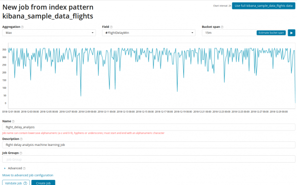
In the field Aggregation you can choose the approach to anomaly detection. For example, with Min values below typical levels will be considered anomalous. There are also Max, High Mean, Low, Mean, Distinct and others. A description of all functions can be found .
In the field Field specifies the numeric field in the document by which we will conduct the analysis.
In the field is the granularity of intervals on the timeline for the analysis. You can trust the automation or select manually. The image below shows an example of too low granularity — you may miss an anomaly. This setting can adjust the algorithm's sensitivity to anomalies.
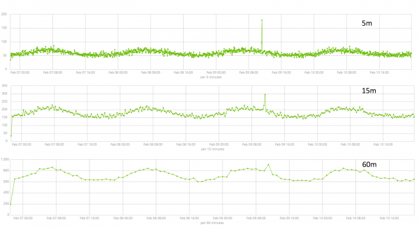
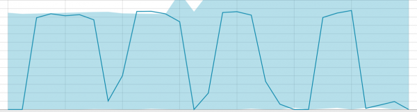
The duration of collected data is a key factor that influences the effectiveness of the analysis. In the analysis, the algorithm identifies repeating intervals, calculates the confidence interval (baseline), and detects anomalies — atypical deviations from the usual behavior of the metric. Just for example:
Baseline for small data segments:
When the algorithm has something to learn from, the baseline looks like this:
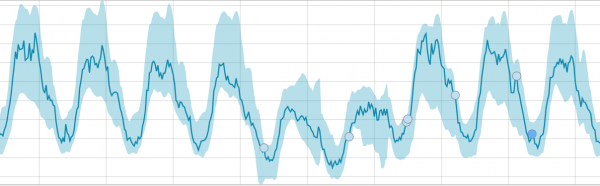
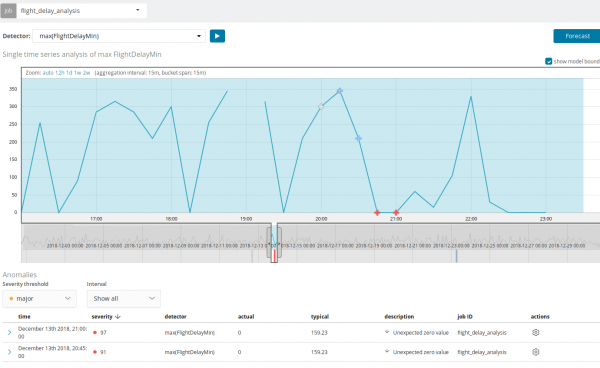
After the task is launched, the algorithm identifies anomalous deviations from the norm and ranks them by anomaly probability (the color of the corresponding label is indicated in parentheses):
Warning (blue): less than 25
Minor (yellow): 25-50
Major (orange): 50-75
Critical (red): 75-100
The graph below shows an example with identified anomalies.
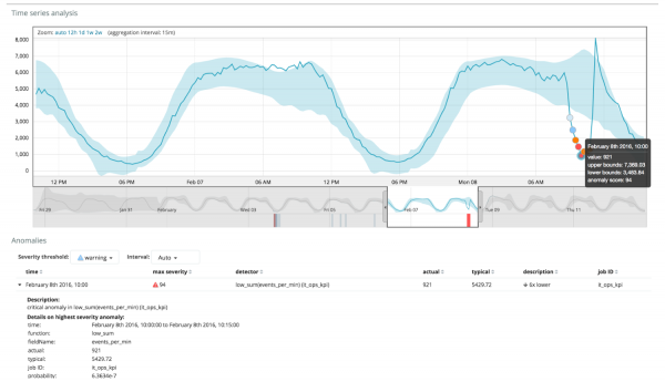
Here we see the number 94, which indicates the probability of an anomaly. It’s clear that since the value is close to 100, this is an anomaly. The column under the graph indicates a negligible probability of 0.000063634% of the metric value appearing there.
In addition to anomaly detection in Kibana, you can run forecasting. This is done easily from the same view with anomalies — click the Forecast button in the upper right corner.
The forecast is built a maximum of 8 weeks ahead. Even if you wish for more, it's not possible by design.
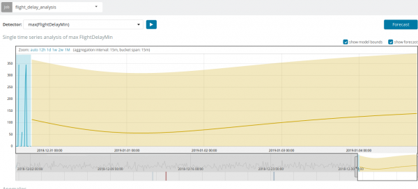
In some cases, forecasting will be very useful, for example, when monitoring user load on infrastructure.
Multi Metric
Next, we move to another ML capability in the Elastic Stack — analyzing multiple metrics as a batch. However, this does not mean that the dependence of one metric on another will be analyzed. It's the same as Single Metric, just with multiple metrics on one screen for easy comparison of their influence on each other. We will discuss the analysis of the dependence of one metric on another in the Population section.
After clicking on the square with Multi Metric, a settings window will appear. Let's take a closer look at these settings.
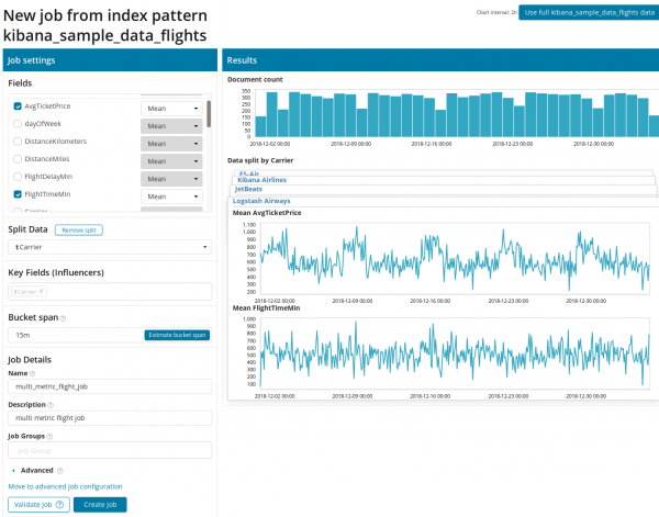
First, you need to select fields for analysis and aggregate data on them. The aggregation options here are the same as for Single Metric (Max, High Mean, Low, Mean, Distinct and others). Next, data can be split by one of the fields if desired (field Split Data). In the example, we did this by the field OriginAirportID. Note that the metrics graph on the right is now presented as multiple graphs.
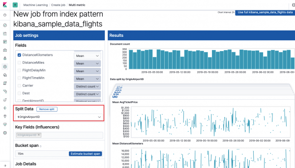
Field Key Fields (Influencers) directly affect the identified anomalies. By default, there will always be at least one value here, and you can add more. The algorithm will take these fields into account during analysis and show the most "influential" values.
After running, the interface in Kibana will look something like this.
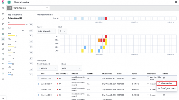
This is the so-called heatmap of anomalies for each value of the field OriginAirportID, which we specified in Split DataAs with Single Metric, the color indicates the level of anomalous deviation. A similar analysis can conveniently be performed, for example, on workstations to monitor those with suspiciously high logins, etc. We have previously written , which can also be collected and analyzed here.
Under the heat map, there is a list of anomalies, each of which can be clicked to access the Single Metric view for detailed analysis.
Population
To search for anomalies among correlations between different metrics in Elastic Stack, there is a specialized Population analysis. It is precisely through this that anomalous values in the performance of a server can be explored in relation to others when, for example, the number of requests to the target system increases.
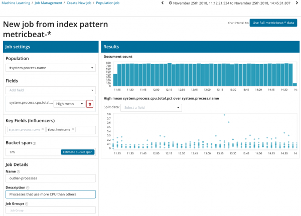
In this illustration, the Population field shows the value to which the analyzed metrics will relate. In this case, it is the process name. As a result, we will see how the CPU load of each of the processes influenced each other.
Note that the graph of the analyzed data differs from those with Single Metric and Multi Metric. This is done in Kibana by design for improved perception of the distribution of the analyzed data values.
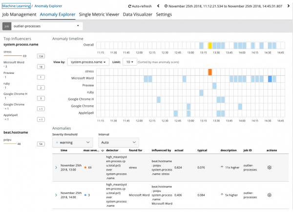
The graph shows that the process behaved anomalously stress (by the way, generated by a special utility) on the server poipu, which influenced (or was an influencer of) the emergence of this anomaly.
Advanced
Analytics with fine-tuning. When performing an Advanced analysis in Kibana, additional settings appear. After clicking on the creation menu on the Advanced tile, a window with tabs appears. The tab Job Details was intentionally skipped; it contains basic settings not directly related to the analysis configuration.
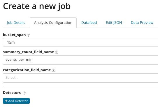
In summary_count_field_name optionally allows specifying the name of the field from the documents that contains aggregated values. In this example — the number of events per minute. In the , the name of the field from the document that contains some variable value is specified. This field can be used as a mask to break down the analyzed data into subsets. Note the button Add detector in the previous illustration. Below is the result of clicking this button.
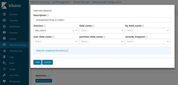
Here is an additional settings block for configuring the anomaly detector for a specific task. We plan to discuss specific use cases (especially related to security) in upcoming articles. For example, one of the discussed cases. It relates to finding rarely occurring values and is implemented .
In the field function you can choose a specific function for anomaly detection. Besides rare, there are a couple of interesting functions — . They uncover anomalies in metric behavior over the course of a day or week, respectively. Other analysis functions .
In field_name specifies the field of the document to be analyzed. By_field_name can be used to split the analysis results by each individual value of the specified document field. If you fill in over_field_name you will get a population analysis, which we discussed earlier. If a value is specified in partition_field_name, separate baselines will be calculated for each value based on this document field (for example, the server name or the process name on the server can act as a value). In exclude_frequent you can select all or none, which will mean excluding (or including) frequently occurring document field values.
In this article, we tried to provide a concise overview of machine learning capabilities in the Elastic Stack, leaving out many details. Let us know in the comments what cases you have solved using the Elastic Stack and for what tasks you use it. To contact us, you can use direct messages on Habr or .
Source: habr.com
