

In the second part of the article on computer system simulators, I will continue to talk in a simple introductory form about computer simulators, namely the full-platform simulation that the average user encounters most often, as well as the per-cycle model and traces that are more common in development circles.

В I talked about what simulators are in general, as well as about the levels of simulation. Now, based on that knowledge, I propose to dive a little deeper and talk about full-platform simulation, how to assemble traces, what to do with them later, and also about clock-based microarchitecture emulation.
Full platform simulator, or “One in the field is not a warrior”
If you want to investigate the operation of one specific device, for example, a network card, or write firmware or a driver for this device, then such a device can be modeled separately. However, using it in isolation from the rest of the infrastructure is not very convenient. To run the corresponding driver, you will need a central processor, memory, access to the bus for data transfer, and so on. In addition, an operating system (OS) and a network stack are required for the driver to work. In addition, a separate packet generator and response server may be required.
A full platform simulator creates an environment to run a complete software stack, which includes everything from the BIOS and bootloader to the OS itself and its various subsystems, such as the same network stack, drivers, user-level applications. To do this, it implements software models of most computer devices: processor and memory, disk, input-output devices (keyboard, mouse, display), as well as the same network card.
Below is a block diagram of the x58 chipset from Intel. A full-platform computer simulator based on this chipset requires the implementation of most of the listed devices, including those that are inside the IOH (Input/Output Hub) and ICH (Input/Output Controller Hub), which are not drawn in detail on the block diagram. Although, as practice shows, there are not so few devices that are not used by the software that we are going to launch. Models of such devices can not be created.
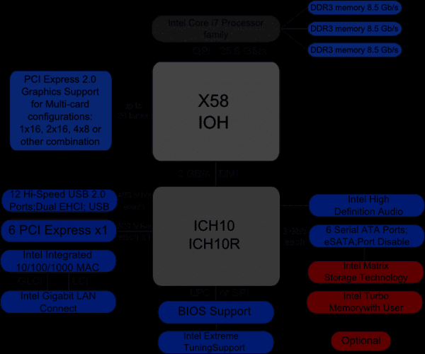
Most often, full-platform simulators are implemented at the processor instruction level (ISA, see below). ). This allows you to relatively quickly and inexpensively create the simulator itself. The ISA level is also good in that it stays more or less constant, as opposed to, for example, the API/ABI level, which changes more frequently. In addition, the implementation at the instruction level allows you to run the so-called unmodified binary software, that is, run the already compiled code without any changes, exactly as it is used on real hardware. In other words, you can make a copy ("dump") of the hard drive, specify it as an image for the model in the full-platform simulator, and - voila! – The OS and other programs are loaded in the simulator without any additional steps.
Simulator performance

As mentioned just above, the very process of simulating the entire system, that is, all its devices, is a rather slow undertaking. If you also implement all this at a very detailed level, for example, microarchitectural or logical, then the execution will become extremely slow. But the instruction level is a good choice and allows the OS and programs to run at speeds sufficient for the user to comfortably interact with them.
Here, it would be appropriate to touch on the topic of simulator performance. Usually it is measured in IPS (instructions per second), more precisely in MIPS (millions IPS), that is, the number of processor instructions executed by the simulator in one second. At the same time, the simulation speed also depends on the performance of the system on which the simulation itself is running. Therefore, perhaps it is more correct to speak of a “slowdown” of the simulator compared to the original system.
The most common full-platform simulators on the market, such as QEMU, VirtualBox or VmWare Workstation, have good performance. It may not even be noticeable to the user that the work is going on in the simulator. This is due to the special virtualization capabilities implemented in processors, binary translation algorithms, and other interesting things. This is all a topic for a separate article, but in a nutshell, virtualization is a hardware feature of modern processors that allows simulators not to simulate instructions, but to execute them directly to a real processor, if, of course, the architectures of the simulator and processor are similar. Binary translation is the translation of the guest machine code into the host code and subsequent execution on a real processor. As a result, the simulation is only slightly slower, about 5-10 times, and often even runs at the same speed as the real system. Although many factors influence this. For example, if we want to simulate a system with several tens of processors, then the speed will immediately drop by these several tens of times. On the other hand, simulators like Simics in recent versions support multiprocessor host hardware and effectively parallelize the simulated cores to the cores of the real processor.
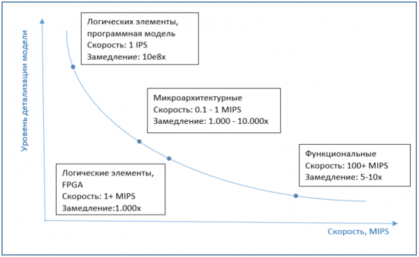
If we talk about the speed of microarchitectural simulation, then it is usually several orders of magnitude, about 1000-10000 times slower than running on a conventional computer, without simulation. And implementations at the level of logical elements are several orders of magnitude slower. Therefore, FPGA is used as an emulator at this level, which can significantly increase performance.
The graph below shows an approximate relationship between simulation speed and model detail.
Clockwise simulation
Despite the low execution speed, microarchitectural simulators are quite common. Simulation of the internal blocks of the processor is necessary in order to accurately simulate the execution time of each instruction. Misunderstanding may arise here - after all, it would seem, why not just take and program the execution time for each instruction. But such a simulator will work very inaccurately, since the execution time of the same instruction may differ from call to call.
The simplest example is a memory access instruction. If the requested memory location is available in the cache, then the execution time will be minimal. If this information is not in the cache (“cache miss”, cache miss), then this will greatly increase the execution time of the instruction. Thus, a cache model is needed for accurate simulation. However, the case is not limited to the cache model. The processor will not simply wait for data to be received from memory when it is not in the cache. Instead, it will start executing the next instructions, choosing those that do not depend on the result of reading from memory. This so-called out-of-order execution (OOO) is required to minimize CPU idle time. To take all this into account when calculating the execution time of instructions, modeling of the corresponding processor blocks will help. Among these instructions, which are executed while waiting for the result of reading from memory, there may be a conditional branch operation. If the result of the condition is unknown at the moment, then again, the processor does not stop execution, but makes a “guess”, executes the appropriate jump, and continues proactively executing the instructions from the jump. Such a block, called a branch predictor, must also be implemented in a microarchitecture simulator.
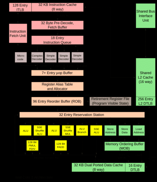
The picture below shows the main blocks of the processor, it is not necessary to know it, it is provided only to show the complexity of the microarchitectural implementation.
The operation of all these blocks in a real processor is synchronized by special clock signals, the same happens in the model. Such a microarchitectural simulator is called cycle accurate. Its main purpose is to accurately predict the performance of the developed processor and / or calculate the execution time of a certain program, for example, a benchmark. If the values are lower than necessary, then it will be necessary to refine the algorithms and processor units or optimize the program.
As shown above, cycle-by-cycle simulation is very slow, so it is used only when studying certain moments of the program's operation, where it is necessary to find out the real speed of program execution and evaluate the future performance of the device whose prototype is being simulated.
At the same time, a functional simulator is used to simulate the rest of the program's operation. How does this combined use actually happen? First, a functional simulator is launched, on which the OS and everything necessary to run the program under study are loaded. After all, we are not interested in either the OS itself, or the initial stages of launching the program, its configuration, and so on. However, we cannot skip these parts and immediately proceed to the execution of the program from the middle. Therefore, all these preliminary steps are run on a functional simulator. After the program has been executed up to the moment of interest to us, two options are possible. You can change the model to cycle-by-cycle and continue execution. A simulation mode that uses executable code (that is, regular compiled program files) is called execution driven simulation. This is the most common simulation option. Another approach is also possible - trace-driven simulation.
Trace-Based Simulation
It consists of two steps. With the help of a functional simulator or on a real system, a log of program actions is collected and written to a file. Such a log is called a trace. Depending on what is being examined, the trace may include executable instructions, memory addresses, port numbers, interrupt information.
The next step is to "play" the trace, where the per-cycle simulator reads the trace and executes all the instructions written in it. At the end, we get the execution time of this piece of the program, as well as various characteristics of this process, for example, the cache hit percentage.
An important feature of working with traces is determinism, that is, by running the simulation in the manner described above, over and over again we reproduce the same sequence of actions. This makes it possible, by changing the parameters of the model (sizes of the cache, buffers and queues) and using different internal algorithms or tuning them, to explore how one or another parameter affects the performance of the system and which option gives the best results. All of this can be done with a device prototype model prior to building a real hardware prototype.
The complexity of this approach lies in the need to pre-run the application and collect the trace, as well as the huge file size with the trace. The advantages include the fact that it is enough to simulate only the part of the device or platform of interest, while simulation by execution requires, as a rule, a complete model.
So, in this article, we looked at the features of full-platform simulation, talked about the speed of implementations at different levels, cycle-by-cycle simulation and traces. In the next article, I will describe the main scenarios for using simulators, both for personal purposes and from the point of view of development in large companies.
Source: habr.com
