

Today we will begin studying the EIGRP protocol, which, along with studying OSPF, is one of the most important topics in the CCNA course.
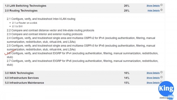
Later we will return to section 2.5, but for now, right after section 2.4, we will move on to section 2.6 "Configuration, verification, and troubleshooting of EIGRP for IPv4 (excluding authentication, filtering, manual summarization, redistribution, and stub configuration)."
Today we will have an introductory lesson where I will tell you about the concept of the Enhanced Interior Gateway Routing Protocol (EIGRP), and in the next two lessons, we will cover the configuration and troubleshooting of this protocol. But first, I want to share the following with you.
In the last few lessons, we studied OSPF. Now I want you to remember that months ago when we studied the RIP protocol, we talked about routing loops and technologies that prevent traffic from looping. How can you prevent routing loops when using OSPF? Can methods like Route Poison or Split Horizon be used for this purpose? These are questions you should answer on your own. You may use other thematic resources, but find the answers to these questions. I want you to learn how to find answers independently, working with various sources, and I will ask you to leave your comments under this video so that I can see how many of my students managed to complete this task.
What is EIGRP? It is a hybrid routing protocol that combines the beneficial features of both distance-vector protocols, like RIP, and link-state protocols, such as OSPF.
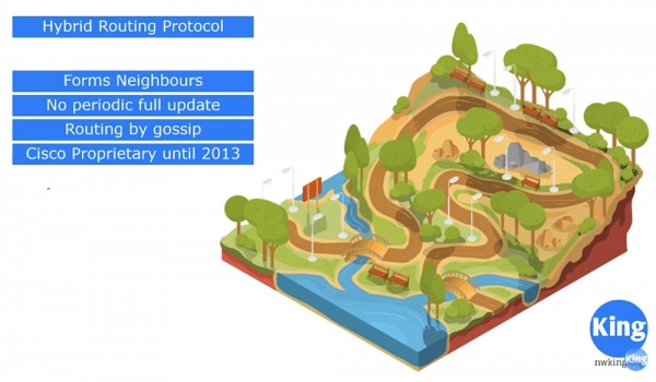
EIGRP is a proprietary protocol of Cisco that was made available for public use in 2013. From the link-state protocol, it adopted the neighbor establishment algorithm, unlike RIP, which does not create neighbors. RIP also exchanges routing tables with other protocol participants, while OSPF, before starting such an exchange, forms a neighbor relationship. EIGRP operates in a similar manner.
The RIP protocol performs periodic updates of the complete routing table every 30 seconds and broadcasts information about all interfaces and routes to all its neighbors. EIGRP does not execute periodic complete updates of information; instead, it uses the concept of Hello messages, as OSPF does. Every few seconds, it sends Hello messages to ensure that the neighbor is still 'alive'.
Unlike distance-vector protocols that analyze the entire network topology before making routing decisions, EIGRP, similar to RIP, creates routes based on rumors. When I say 'rumors,' I mean that when a neighbor reports something, EIGRP takes that as absolute truth. For instance, if a neighbor claims to know how to reach 10.1.1.2, EIGRP believes them without asking, 'How do you know that? Tell me about the topology of the entire network!'
Until 2013, if you only used Cisco infrastructure, you could use EIGRP since this protocol was created back in 1994. However, many companies, even using Cisco equipment, did not want to work with this protocol. In my opinion, EIGRP is the best dynamic routing protocol today as it is much easier to use, though people still prefer OSPF. I think this reluctance is because they do not want to 'tie' themselves to Cisco products. However, Cisco made this protocol publicly available because it supports third-party network equipment, like Juniper, and if you partner with a company that does not use Cisco equipment, you won't run into any issues.
Let's take a brief look at the history of network protocols.
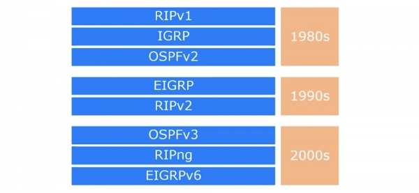
The RIPv1 protocol, which emerged in the 1980s, had several limitations, such as a maximum hop count of 16, which prevented it from providing routing in large networks. Shortly thereafter, the Interior Gateway Routing Protocol IGRP was developed, which was much better than RIP. However, it was more of a distance-vector protocol than a link-state protocol. In the late 80s, an open standard emerged—the OSPFv2 link-state protocol for IPv4.
In the early 90s, Cisco decided that the IGRP protocol needed improvement and released the enhanced interior gateway routing protocol EIGRP. It was much more efficient than OSPF because it combined features of both RIP and OSPF. When we start studying it, you will find that configuring EIGRP is much easier than OSPF. Cisco aimed to create a protocol that would ensure maximum network convergence speed.
In the late 90s, an updated classless version of the RIPv2 protocol was released. In the 2000s, the third version of OSPF, RIPng, and EIGRPv6 appeared, supporting the IPv6 protocol. The world is gradually moving towards a full transition to IPv6, and routing protocol developers want to be ready for it.
As you may recall, we studied that when selecting the optimal route, RIP, as a distance-vector protocol, is guided by just one criterion—the minimum number of hops or minimum distance to the destination interface. Thus, router R1 will choose a direct route to router R3 despite the fact that the speed on this route is 64 kbps, which is much less than the speed on the R1-R2-R3 route, which is 1544 kbps. The RIP protocol will consider the slow one-hop route optimal, rather than the fast two-hop route.
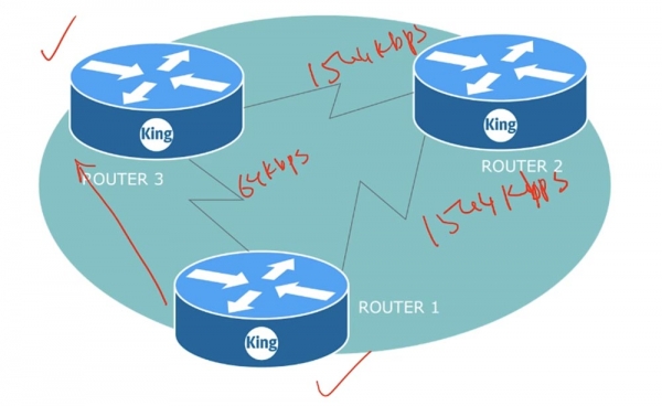
OSPF will examine the entire network topology and decide to connect to router R3 using the route through router R2 as the faster option. The metric for RIP is the number of hops, while OSPF's metric is cost, which is generally proportional to the channel's bandwidth.
EIGRP also focuses on route cost; however, its metric is much more complex than OSPF's and relies on several factors, including Bandwidth, Delay, Reliability, Loading, and Maximum Transmission Unit (MTU). For example, if a certain node is more loaded than others, EIGRP will analyze the load across the entire route and select a different node with lower load.
In the CCNA course, we will only consider factors that shape the metric, such as Bandwidth and Delay; these will be used in the metric formula.
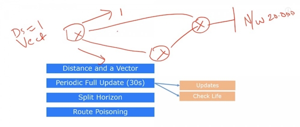
The distance-vector protocol RIP uses two concepts: distance and direction. If we have three routers, and one of them is connected to the network 20.0.0.0, then the selection will be based on distance – which is in hops, in this case, 1 hop – and on the direction, meaning which way to send the traffic – upper or lower.
Additionally, RIP uses periodic information updates by sending the complete routing table across the network every 30 seconds. This update serves two functions. The first is to update the routing table itself, and the second is to check the liveness of the neighbor. If a device does not receive a response with an updated table or new routing information from a neighbor within 30 seconds, it understands that the route to that neighbor can no longer be used. The router sends updates every 30 seconds to check if the neighbor is still 'alive' and if the route is still valid.
As I mentioned, to prevent routing loops, the Split Horizon technique is used. This means that the update is not sent back to the interface from which it came. The second technology to prevent loops is Route Poisoning. If the connection to the network 20.0.0.0, as shown in the picture, is interrupted, the router connected to it sends 'poisoned route' updates to its neighbors, indicating that this network is now reachable in 16 hops, which means it's virtually unreachable. This is how the RIP protocol works.
How does EIGRP work? If you remember from the lessons on OSPF, this protocol performs three functions: it establishes neighbor relationships, updates the LSDB based on changes in network topology using LSA, and builds the routing table. Establishing neighbor relationships is a complex procedure that uses many parameters. For example, checking and modifying the 2WAY connection – some connections remain in a bidirectional state, while others transition to FULL state. Unlike OSPF, in the EIGRP protocol, this does not happen – it checks only 4 parameters.
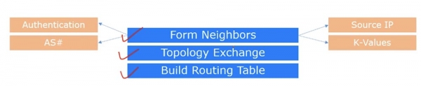
Like OSPF, this protocol sends a Hello message every 10 seconds containing 4 parameters. The first is the authentication criteria, if it has been pre-configured. All devices establishing neighbor relationships must have the same authentication parameters.
The second parameter is used to verify that the devices belong to the same autonomous system, meaning that for neighbor establishment via the EIGRP protocol, both devices must have the same autonomous system number. The third parameter checks that Hello messages are sent from the same source IP address.
The fourth parameter is used to verify the matching of K-Values. The EIGRP protocol uses 5 such coefficients from K1 to K5. If you recall, when K=0, the parameters are ignored; when K=1, the parameters are used in the metric calculation formula. Therefore, the values of K1-5 must be the same for different devices. In the CCNA course, we will accept these coefficients' default values: K1 and K3 equal to 1, while K2, K4, and K5 equal to 0.
Thus, if these 4 parameters match, EIGRP establishes neighbor relationships, and the devices add each other to the neighbor table. Subsequently, changes are made in the topology table.

All Hello messages are sent to the multicast IP address 224.0.0.10, and updates, depending on the configuration, are sent to the unicast addresses of neighbors or to the multicast address. This update uses a different protocol called RTP, Reliable Transport Protocol, or 'Reliable Transport Protocol.' This protocol checks whether the neighbor has received the update, and as its name suggests, its key function is to ensure communication reliability. If the update has not reached the neighbor, the transmission will be repeated until it is received. In OSPF, there is no mechanism to verify the receiving device, so the system does not know whether the neighboring devices received the update.
If you recall, RIP sends updates of the complete network topology every 30 seconds. EIGRP only does this if a new device appears in the network or if there are any changes. If the subnet topology has changed, the protocol will send an update, but not of the entire topology table, only the entries with that change. If a subnet has changed, only its topology will be updated. This looks like a partial update that occurs when needed.
As you know, OSPF sends LSA every 30 minutes regardless of whether any changes have occurred in the network. EIGRP will not send any updates for a long period until some changes occur in the network. Therefore, EIGRP is much more efficient than OSPF.
After the routers exchange update packets, the third stage occurs – forming the routing table based on the metric calculated using the formula shown in the figure. It calculates the cost, and based on this cost, it makes a decision.
Suppose R1 sent a Hello to router R2, and R2 replied with a Hello to router R1. If all parameters match, the routers create a neighbor table. In this table, R2 records an entry for router R1, and R1 creates an entry for R2. After this, router R1 sends an update to the connected network 10.1.1.0/24. In the routing table, this appears as information about the IP address of the network, the router interface that connects to it, and the cost of the route through that interface. If you remember, the cost for EIGRP is 90, and then the Distance value is specified, which we will discuss later.
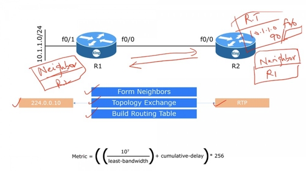
The complete metric formula looks much more complex, as it includes the values of K coefficients and various transformations. The full form of the formula is provided on the Cisco website, but if you substitute the default coefficient values, it simplifies to a more straightforward form – the metric will equal (bandwidth + Delay) * 256.
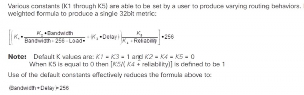
We will use this simplified version of the formula to calculate the metric, where the bandwidth in kilobits is equal to 107 divided by the minimum bandwidth of all interfaces leading to the least-bandwidth destination network, and the cumulative-delay is the total delay in tens of microseconds across all interfaces leading to the destination network.
When studying EIGRP, we must understand four definitions: Feasible Distance, Reported Distance, Successor (the neighboring router with the lowest path cost to the destination network), and Feasible Successor (the backup neighboring router). To grasp their meanings, let's consider the following network topology.
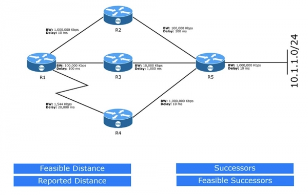
Let's start by creating the routing table for R1 to select the best route to the network 10.1.1.0/24. Next to each device is the bandwidth in kbps and the delay in ms. We are using GigabitEthernet interfaces with a bandwidth of 100 Mbps, or 1000000 kbps, FastEthernet interfaces with a speed of 100000 kbps, Ethernet at 10000 kbps, and a serial interface with a speed of 1544 kbps. These values can be determined by checking the specs of the respective physical interfaces in the router's settings.
The default bandwidth for Serial interfaces is 1544 kbps, and even if you have a 64 kbps line, the bandwidth will still be 1544 kbps. Therefore, as a network administrator, you need to ensure that you are using the correct bandwidth value. For a specific interface, it can be set using the bandwidth command, and the delay can be modified from its default value using the delay command. You don’t need to worry about default bandwidth values for GigabitEthernet or Ethernet interfaces, but be cautious when selecting line speed if using Serial interfaces.
Note that in this diagram, the delay is indicated as if it were in milliseconds (ms), but in reality, it is in microseconds; I simply do not have the μ character for the correct notation of microseconds (μs).
Pay close attention to the following circumstance. If you enter the command show interface g0/0, the system will display the delay in tens of microseconds, not just in microseconds.
We will discuss this issue in detail in the next video dedicated to EIGRP configuration. For now, remember that when substituting delay values in the formula, 100 μs turns into 10, since the formula uses tens of microseconds, not single units.
In the diagram, I will mark the interfaces related to the shown bandwidths and delays with red dots.
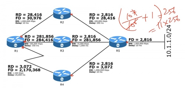
First, we need to determine the possible Feasible Distance. This is the FD metric, calculated using a formula. For the segment from R5 to the external network, we need to divide 107 by 106, resulting in 10. Next, we must add the delay, which is equal to 1, since we have 10 microseconds, or one decade. Therefore, the resulting value of 11 should be multiplied by 256, making the metric value 2816. This is the FD value for this segment of the network.
This value will be sent by router R5 to router R2, becoming the Reported Distance (RD) for R2, which is the value reported by its neighbor. Thus, the declared distance (RD) for all other devices will equal the possible distance (FD) of the device reporting it.
Router R2 calculates FD based on its data, dividing 107 by 105 to get 100. It then adds the sum of the delays on the route to the external network: R5's delay, which is one decade of microseconds, and its own delay, which is ten decades. The total delay will be 11 decades of microseconds. Adding it to the obtained hundred gives us 111, multiplying this by 256 gives us FD=28416. Similarly, router R3 ends up with FD=281856 after its calculations. Router R4 calculates FD=3072 and sends it to R1 as RD.
Note that router R1, when calculating FD, substitutes not its own bandwidth of 1000000 kbps into the formula, but the lower bandwidth of router R2, which is 100000 kbps, because the formula always uses the minimum bandwidth of the interface leading to the destination network. In this case, on the path to the 10.1.1.0/24 network, there are routers R2 and R5, but since the bandwidth of the fifth router is higher, the formula uses the lowest value of router R2’s bandwidth. The total delay on the R1-R2-R5 path is 1+10+1 (tens) = 12, the reported bandwidth is 100, and the sum of these numbers multiplied by 256 will give the value FD=30976.
So, all devices have calculated the FD of their interfaces, and router R1 has 3 routes leading to the destination network. These are the routes R1-R2, R1-R3, and R1-R4. The router selects the minimum possible distance FD, which is 30976 – this is the route to router R2. This router becomes the Successor. The routing table also indicates a Feasible Successor – it means that in the event of a link failure between R1 and the Successor, the route will be through the backup router Feasible Successor.
Feasible Successors are appointed according to a single rule: the reported distance RD of this router must be less than the FD of the router on the segment to the Successor. In our case, R1-R2 has FD=30976, RD on the R1-K3 segment is 281856, and RD on the R1-R4 segment is 3072. Since 3072 < 30976, router R4 is chosen as the Feasible Successor.
This means that in the event of a link failure on the R1-R2 segment, traffic to the 10.1.1.0/24 network will be routed via R1-R4-R5. Route switching using RIP takes several tens of seconds; with OSPF, it takes a few seconds, while EIGRP switches instantly. This is another advantage of EIGRP over other routing protocols.
What happens if the connection with both the Successor and Feasible Successor is interrupted at the same time? In this case, EIGRP will invoke the DUAL algorithm, which can compute a backup route through the likely successor. This may take a few seconds, during which EIGRP will find another neighbor that can be used for traffic transmission and place its data in the routing table. After that, the protocol will continue its regular routing operations.
Thank you for staying with us. Do you enjoy our articles? Would you like to see more interesting materials? Support us by placing an order or recommending us to your friends. 30% discount for Habr users on a unique entry-level server designed by us for you: (options available with RAID1 and RAID10, up to 24 cores and up to 40GB DDR4).
Dell R730xd for half the price? Only with us in the Netherlands! Dell R420 — 2x E5-2430 2.2GHz 6C 128GB DDR3 2x960GB SSD 1Gbps 100TB — from $99! Read about how
Source: habr.com
