

A Brief Introduction
I believe that we could accomplish more tasks if we were provided with step-by-step instructions that tell us what to do and how to do it. I recall moments in my life when I couldn't start something because it was simply hard to understand where to begin. Perhaps, a long time ago, you saw the words 'Data Science' on the internet and thought it was far beyond your reach, that the people working in this field were somewhere else, in another world. But no, they are right here. And perhaps thanks to someone in this field, an article caught your attention in your feed. There are plenty of courses that can help you get a grip on this craft, and here I will help you take the first step.
So, are you ready? Let me tell you right away that you'll need to know Python 3, as I will be using it here. I also recommend that you install Jupyter Notebook in advance or check how to use Google Colab.
Step One

Kaggle is your significant ally in this endeavor. In principle, you can manage without it, but I will discuss that in another article. It is a platform where Data Science competitions are hosted. In each competition, at the early stages, you will gain an incredible amount of experience solving various types of tasks, development experience, and teamwork experience, which is crucial in today's world.
We will take our task from there. It is titled as follows: 'Titanic'. The condition is to predict whether each individual will survive. In general terms, the task of someone involved in Data Science is data collection, processing, model training, prediction, and so on. Kaggle allows us to skip the data collection phase—it's available on the platform. We need to download it, and then we can start working!
You can do this as follows:
In the Data tab, you will find the files containing the data.


We have uploaded the data, prepared our Jupyter notebooks, and…
Step Two
How do we now load this data?
First, we import the necessary libraries:
import pandas as pd
import numpy as np
Pandas will allow us to load .csv files for further processing.
NumPy is needed to represent our data table as a matrix of numbers.
Let's move on. We will take the train.csv file and load it:
dataset = pd.read_csv('train.csv')
We will refer to our sample train.csv data through the variable dataset. Let's take a look at what is there:
dataset.head()

The head() function allows us to view the first few rows of the dataframe.
The Survived column represents our results, which are known in this dataframe. Regarding the task, we need to predict the Survived column for the test.csv data. This data contains information about other Titanic passengers for whom we do not know the outcomes.
So, let's divide our table into dependent and independent data. It’s quite simple. Dependent data is what depends on independent data — what is present in the outcomes. Independent data is what influences the outcome.
For example, we have this dataset:
"Vova studied computer science — no.
Vova received a grade of 2 in computer science."
The grade in computer science depends on the answer to the question: did Vova study computer science? Clear? Let's proceed, we are getting closer to the goal!
The traditional variable for independent data is X. For dependent data — y.
We will do the following:
X = dataset.iloc[ : , 2 : ]
y = dataset.iloc[ : , 1 : 2 ]
What is this? With the function iloc[:, 2: ] we tell Python: I want to see in variable X the data starting from the second column (inclusive, assuming the count starts at zero). In the second line, we indicate that we want to see in y the data from the first column.
[ a:b, c:d ] — this is the construct we are using in the brackets. If we do not specify any variables, they will be kept as default. That is, we can specify [:,: d] and then we will get all columns in the dataframe except for those starting from number d and onwards. The variables a and b define the rows, but we need all of them, so we leave that default.
Let's see what we have:
X.head() 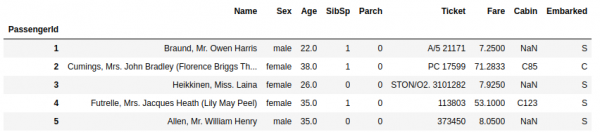
y.head() 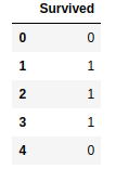
To simplify this brief lesson, we will remove the columns that require special "care", or that do not influence survival at all. They contain string type data.
count = ['Name', 'Ticket', 'Cabin', 'Embarked']
X.drop(count, inplace=True, axis=1)
Great! Let's move on to the next step.
Step three
Here we need to encode our data so that the machine can better understand how this data affects the outcome. However, we will encode only certain data types, specifically the 'Sex' column. How do we want to encode it? Let's represent the gender information as a vector: 10 for male and 01 for female.
First, let's convert our tables into a NumPy matrix:
X = np.array(X)
y = np.array(y)
And now let's take a look:
from sklearn.compose import ColumnTransformer
from sklearn.preprocessing import OneHotEncoder

ct = ColumnTransformer(transformers=[('encoder', OneHotEncoder(), [1])],
                       remainder='passthrough')
X = np.array(ct.fit_transform(X))
The sklearn library is a fantastic library that allows us to perform comprehensive work in Data Science. It contains a large number of interesting machine learning models, as well as tools for data preparation.
OneHotEncoder will allow us to encode a person's gender in the way we described. Two classes will be created: male and female. If a person is male, a 1 will be recorded in the 'male' column, and a 0 in the 'female' column.
After OneHotEncoder(), the [1] signifies that we want to encode column number 1 (counting starts at zero).
Great. Let's move further!
Typically, situations arise where some data remains unfilled (i.e., NaN — not a number). For example, we have information about a person: their name and gender. However, there is no data about their age. In this case, we will use a method: we will find the arithmetic mean across all columns, and if some data in any column is missing, we will fill in the gap with the arithmetic mean.
from sklearn.impute import SimpleImputer
imputer = SimpleImputer(missing_values=np.nan, strategy='mean')
imputer.fit(X)
X = imputer.transform(X)
Now let's consider that there are situations when data is very widely spread. Some data points are within [0:1], while others may reach hundreds or thousands. To mitigate this spread and allow the computer to be more accurate in its calculations, we will scale the data. Let's ensure all numbers do not exceed three. For this, we will use the StandardScaler function.
from sklearn.preprocessing import StandardScaler
sc = StandardScaler()
X[:, 2:] = sc.fit_transform(X[:, 2:])
Now our data looks like this:

Class. We are already close to our goal!
Step four
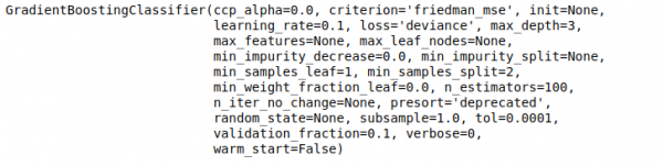
Let's train our first model! The sklearn library offers a vast array of interesting tools. I applied the Gradient Boosting Classifier model to this task. We use a classifier because our goal is a classification task. We need to predict whether the outcome is 1 (survived) or 0 (did not survive).
from sklearn.ensemble import GradientBoostingClassifier
gbc = GradientBoostingClassifier(learning_rate=0.5, max_depth=5, n_estimators=150)
gbc.fit(X, y)
The fit function tells Python: Let the model discover the relationships between X and y.
In less than a second, the model is ready.
How do we apply it? We will see now!
Step five. Conclusion
Now we need to load the table with our test data for which we need to make predictions. We will perform the same actions with this table that we did for X.
X_test = pd.read_csv('test.csv', index_col=0)

count = ['Name', 'Ticket', 'Cabin', 'Embarked']
X_test.drop(count, inplace=True, axis=1)

X_test = np.array(X_test)

from sklearn.compose import ColumnTransformer
from sklearn.preprocessing import OneHotEncoder
ct = ColumnTransformer(transformers=[('encoder', OneHotEncoder(), [1])],
                       remainder='passthrough')
X_test = np.array(ct.fit_transform(X_test))

from sklearn.impute import SimpleImputer
imputer = SimpleImputer(missing_values=np.nan, strategy='mean')
imputer.fit(X_test)
X_test = imputer.transform(X_test)

from sklearn.preprocessing import StandardScaler
sc = StandardScaler()
X_test[:, 2:] = sc.fit_transform(X_test[:, 2:])
Let’s apply our model now!
gbc_predict = gbc.predict(X_test)
Done. We created the predictions. Now we need to save them to a CSV file and upload it to the website.
np.savetxt('my_gbc_predict.csv', gbc_predict, delimiter=",", header = 'Survived')
All set. We received a file containing predictions for each passenger. All that's left is to upload these solutions to the website and evaluate the forecast. This simple solution provides not only 74% correct answers in public datasets but also a boost in Data Science. The most curious can always message me privately with questions. Thank you all!
Source: habr.com
