

As we approach the start of the course we have prepared another useful translation for you.
Graph databases are an essential technology for database specialists. I strive to keep an eye on innovations and new technologies in this field, and after working with both relational and NoSQL databases, I see that the role of graph databases is becoming increasingly significant. When dealing with complex hierarchical data, traditional databases and even NoSQL often prove inefficient. Typically, as the number of levels in connections and the size of the database increase, performance tends to decrease. Moreover, as the complexity of relationships grows, the number of JOINs also increases.
Of course, there are solutions for working with hierarchies in the relational model (such as using recursive CTEs), but these remain workarounds. In contrast, the graph database capabilities of SQL Server allow for easy management of multiple levels of hierarchy. This simplifies both the data model and the queries, thereby enhancing their efficiency and significantly reducing the amount of code.
Graph databases are an expressive language for representing complex systems. This technology is already widely used in the IT industry in areas such as social networks, anti-fraud systems, IT network analysis, social recommendations, and product and content recommendations.
The functionality of graph databases in SQL Server is suitable for scenarios in which data is heavily interconnected and has clearly defined relationships.
Graph data model
A graph is a collection of vertices (nodes) and edges (connections). Vertices represent entities, while edges represent relationships, which can contain information in their attributes.
A graph database models entities as a graph as defined by graph theory. The data structures are vertices and edges. Attributes are the properties of vertices and edges. A connection is the linkage between vertices.
Unlike other data models, graph databases prioritize the relationships between entities. Therefore, there is no need to compute relationships through foreign keys or other means. Complex data models can be created using only the abstractions of vertices and edges.
In today's world, modeling relationships requires increasingly sophisticated techniques. SQL Server 2017 offers graph database capabilities for modeling connections. Nodes and edges of the graph are represented as new types of tables: NODE and EDGE. A new T-SQL function called MATCH() is used to query the graph. Since this functionality is built into SQL Server 2017, you can use it in your existing databases without any need for conversion.
Benefits of the Graph Model
Currently, businesses and users demand applications that handle larger and larger volumes of data, expecting high performance and reliability. Representing data as a graph provides convenient means for processing complex relationships. This approach helps solve many problems and aids in obtaining results within a given context.
It seems that many applications will benefit from the use of graph databases in the future.
Data Modeling: From Relational Model to Graph
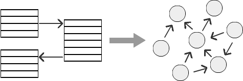
Example
Let’s consider an example of an organizational structure with a hierarchy of employees: an employee reports to a manager, the manager reports to a senior manager, and so on. Depending on the specific company, this hierarchy can have any number of levels. However, as the number of levels increases, calculating relationships in a relational database becomes increasingly complex. It is quite challenging to represent an employee hierarchy, marketing hierarchy, or social network connections. Let’s see how SQL Graph can address the issue of handling different levels of hierarchy.
For this example, we will create a simple data model. We will create an employee table. EMP with an identifier EMPNO and a column MGR, indicating the identifier of the employee's manager. All information about the hierarchy is stored in this table and can be queried using the columns. EMPNO and MGR.
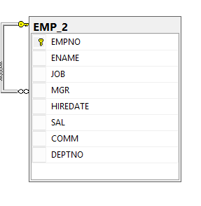
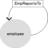
The next diagram shows the same organizational structure model with four levels of nesting in a more familiar form. Employees are the nodes of the graph from the table. EMPThe entity 'employee' is linked to itself with the relationship 'reports to' (ReportsTo). In graph terms, a relationship is an edge (EDGE) that connects the nodes (NODE) of employees.
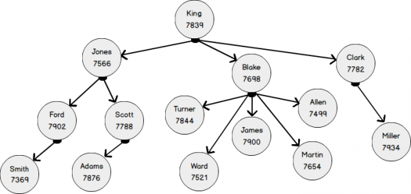
Let's create a simple table EMP and add values according to the diagram above.
CREATE TABLE EMP
(EMPNO INT NOT NULL,
ENAME VARCHAR(20),
JOB VARCHAR(10),
MGR INT,
JOINDATE DATETIME,
SALARY DECIMAL(7, 2),
COMMISIION DECIMAL(7, 2),
DNO INT)

INSERT INTO EMP VALUES
(7369, 'SMITH', 'CLERK', 7902, '02-MAR-1970', 8000, NULL, 2),
(7499, 'ALLEN', 'SALESMAN', 7698, '20-MAR-1971', 1600, 3000, 3),
(7521, 'WARD', 'SALESMAN', 7698, '07-FEB-1983', 1250, 5000, 3),
(7566, 'JONES', 'MANAGER', 7839, '02-JUN-1961', 2975, 50000, 2),
(7654, 'MARTIN', 'SALESMAN', 7698, '28-FEB-1971', 1250, 14000, 3),
(7698, 'BLAKE', 'MANAGER', 7839, '01-JAN-1988', 2850, 12000, 3),
(7782, 'CLARK', 'MANAGER', 7839, '09-APR-1971', 2450, 13000, 1),
(7788, 'SCOTT', 'ANALYST', 7566, '09-DEC-1982', 3000, 1200, 2),
(7839, 'KING', 'PRESIDENT', NULL, '17-JUL-1971', 5000, 1456, 1),
(7844, 'TURNER', 'SALESMAN', 7698, '08-AUG-1971', 1500, 0, 3),
(7876, 'ADAMS', 'CLERK', 7788, '12-MAR-1973', 1100, 0, 2),
(7900, 'JAMES', 'CLERK', 7698, '03-NOV-1971', 950, 0, 3),
(7902, 'FORD', 'ANALYST', 7566, '04-MAR-1961', 3000, 0, 2),
(7934, 'MILLER', 'CLERK', 7782, '21-JAN-1972', 1300, 0, 1)
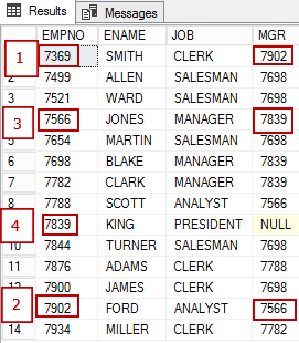
The employees shown in the diagram below are:
- the employee with EMPNO 7369 reports to 7902;
- the employee with EMPNO 7902 reports to 7566
- the employee with EMPNO 7566 reports to 7839
Now let's look at the representation of the same data as a graph. The vertex EMPLOYEE has several attributes and is self-referential with the 'reports to' relationship (EmplReportsTo). EmplReportsTo is the name of the relationship.
The edge table (EDGE) can also have attributes.
Let's create the node table EmpNode
The syntax for creating a node is quite simple: to the statement CREATE TABLE you add 'AS NODE'.
CREATE TABLE dbo.EmpNode(
ID Int Identity(1,1),
EMPNO NUMERIC(4) NOT NULL,
ENAME VARCHAR(10),
MGR NUMERIC(4),
DNO INT
) AS NODE;
Now we will transform data from a regular table into a graph format. The following INSERT inserts data from the relational table EMP.
INSERT INTO EmpNode(EMPNO,ENAME,MGR,DNO) select empno,ename,MGR,dno from emp 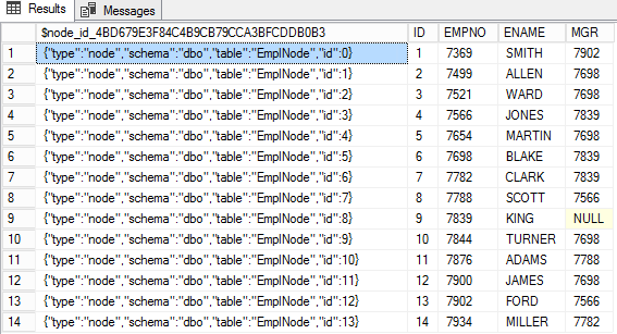
In the node table, a special column $node_id_* stores the node identifier in JSON format. Other columns in this table contain node attributes.
Creating edges (EDGE)
Creating an edge table is very similar to creating a node table, except that the keyword used is 'AS EDGE'.
CREATE TABLE empReportsTo(Deptno int) AS EDGE 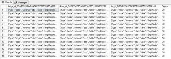
Now, let's define relationships between employees using the columns EMPNO and MGR. The organizational chart clearly shows how to write INSERT.
INSERT INTO empReportsTo VALUES ((SELECT $node_id FROM EmpNode WHERE ID = 1),
   	(SELECT $node_id FROM EmpNode WHERE id = 13),20);
INSERT INTO empReportsTo VALUES ((SELECT $node_id FROM EmpNode WHERE ID = 2),
   	(SELECT $node_id FROM EmpNode WHERE id = 6),10);
INSERT INTO empReportsTo VALUES ((SELECT $node_id FROM EmpNode WHERE ID = 3),
   	(SELECT $node_id FROM EmpNode WHERE id = 6),10)
INSERT INTO empReportsTo VALUES ((SELECT $node_id FROM EmpNode WHERE ID = 4),
   	(SELECT $node_id FROM EmpNode WHERE id = 9),30);
INSERT INTO empReportsTo VALUES ((SELECT $node_id FROM EmpNode WHERE ID = 5),
   	(SELECT $node_id FROM EmpNode WHERE id = 6),30);
INSERT INTO empReportsTo VALUES ((SELECT $node_id FROM EmpNode WHERE ID = 6),
   	(SELECT $node_id FROM EmpNode WHERE id = 9),30);
INSERT INTO empReportsTo VALUES ((SELECT $node_id FROM EmpNode WHERE ID = 7),
   	(SELECT $node_id FROM EmpNode WHERE id = 9),30);
INSERT INTO empReportsTo VALUES ((SELECT $node_id FROM EmpNode WHERE ID = 8),
   	(SELECT $node_id FROM EmpNode WHERE id = 4),30);
INSERT INTO empReportsTo VALUES ((SELECT $node_id FROM EmpNode WHERE ID = 9),
   	(SELECT $node_id FROM EmpNode WHERE id = 9),30);
INSERT INTO empReportsTo VALUES ((SELECT $node_id FROM EmpNode WHERE ID = 10),
   	(SELECT $node_id FROM EmpNode WHERE id = 6),30);
INSERT INTO empReportsTo VALUES ((SELECT $node_id FROM EmpNode WHERE ID = 11),
   	(SELECT $node_id FROM EmpNode WHERE id = 8),30);
INSERT INTO empReportsTo VALUES ((SELECT $node_id FROM EmpNode WHERE ID = 12),
   	(SELECT $node_id FROM EmpNode WHERE id = 6),30);
INSERT INTO empReportsTo VALUES ((SELECT $node_id FROM EmpNode WHERE ID = 13),
   	(SELECT $node_id FROM EmpNode WHERE id = 4),30);
INSERT INTO empReportsTo VALUES ((SELECT $node_id FROM EmpNode WHERE ID = 14),
   	(SELECT $node_id FROM EmpNode WHERE id = 7),30);
The default edge table consists of three columns. The first, $edge_id — identifies the edge in JSON. The other two ($from_id and $to_id) represent the connection between nodes. Additionally, edges can have extra properties. In our case, these are Deptno.
System views
In the system view sys.tables two new columns were added:
- is_edge
- is_node
SELECT t.is_edge, t.is_node,*
FROM sys.tables t
WHERE name like 'emp%' 
SSMS
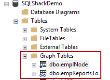
Graph-related objects are located in the Graph Tables folder. The node table icon is marked with a dot, while the edge tables are represented by two connected circles (similar to glasses).
The MATCH expression
Expression MATCH is derived from CQL (Cypher Query Language). This is an efficient way to query graph properties. CQL starts with the expression MATCH.
Syntax
MATCH ()

::=
    { {
                 	{ <-()- }
               	| { -()-> }

             	}
 	}
 	[ { AND } { () } ]
 	[ ,...n ]

::=
    node_table_name | node_alias

::=
    edge_table_name | edge_alias
Examples
Let's look at a few examples.
The query below displays employees reporting to Smith and his manager.
SELECT
E.EMPNO, E.ENAME, E.MGR, E1.EMPNO, E1.ENAME, E1.MGR
FROM
    empnode e, empnode e1, empReportsTo m
WHERE
    MATCH(e-(m)->e1)
and e.ENAME='SMITH' 
The following query is intended to find second-level employees and managers for Smith. If the clause is removed, WHEREthen all employees will be displayed in the result.
SELECT
E.EMPNO,E.ENAME,E.MGR,E1.EMPNO,E1.ENAME,E1.MGR,E2.EMPNO,e2.ENAME,E2.MGR
FROM
    empnode e, empnode e1, empReportsTo m ,empReportsTo m1, empnode e2
WHERE
    MATCH(e-(m)->e1-(m1)->e2)
and e.ENAME='SMITH' 
And finally, the query for third-level employees and managers.
SELECT
E.EMPNO,E.ENAME,E.MGR,E1.EMPNO,E1.ENAME,E1.MGR,E2.EMPNO,e2.ENAME,E2.MGR,E3.EMPNO,e3.ENAME,E3.MGR
FROM
    empnode e, empnode e1, empReportsTo m ,empReportsTo m1, empnode e2, empReportsTo M2, empnode e3
WHERE
    MATCH(e-(m)->e1-(m1)->e2-(m2)->e3)
and e.ENAME='SMITH' 
Now let's change direction to find Smith's bosses.
SELECT
E.EMPNO,E.ENAME,E.MGR,E1.EMPNO,E1.ENAME,E1.MGR,E2.EMPNO,e2.ENAME,E2.MGR,E3.EMPNO,e3.ENAME,E3.MGR
FROM
    empnode e, empnode e1, empReportsTo m ,empReportsTo m1, empnode e2, empReportsTo M2, empnode e3
WHERE
MATCH(e<-(m)-e1<-(m1)-e2<-(m2)-e3) 
Conclusion
SQL Server 2017 has established itself as a full-fledged enterprise solution for various IT business tasks. The first version of SQL Graph is very promising. Even with some limitations, there is already enough functionality to explore graph capabilities.
The SQL Graph functionality is fully integrated into the SQL Engine. However, as mentioned, SQL Server 2017 has the following limitations:
No support for polymorphism.
- Only unidirectional relationships are supported.
- The $from_id and $to_id columns of edges cannot be updated through UPDATE.
- Transitive closures are not supported, but they can be obtained using CTE.
- Limited support for In-Memory OLTP objects.
- Temporal tables (System-Versioned Temporal Table), local and global temporary tables are not supported.
- Table types and table variables cannot be declared as NODE or EDGE.
- Cross-database queries are not supported.
- There is no direct way or wizard to convert regular tables into graphs.
- There is no GUI for graph visualization, but Power BI can be used.
Read more:
Source: habr.com
