I am publishing the first chapter of lectures on control theory, after which your life will never be the same again.

Lectures for the course 'Control of Technical Systems,' given by Oleg Stepanovich Kozlov at the 'Nuclear Reactors and Energy Installations' department of the 'Energy Machine Engineering' faculty at Bauman Moscow State Technical University. He deserves great appreciation for this.

These lectures are being prepared for publication as a book, and since there are specialists in TAU, students, and others interested in the subject here, any criticism is welcome.

1. Key Concepts of Control Theory for Technical Systems

1.1. Goals, Principles of Control, Types of Control Systems, Basic Definitions, Examples

The development and improvement of industrial production (energy, transportation, machine engineering, aerospace technology, etc.) require a continuous increase in the performance of machines and units, higher product quality, reduced costs, and, especially in nuclear energy, a sharp increase in safety (nuclear, radiation, etc.) of nuclear power plants and nuclear installations.

The achievement of these goals is impossible without the implementation of modern control systems, including both automated systems (involving human operators) and automatic systems (without human operators).

Definition: Control is the organization of a particular technological process that ensures the achievement of the set goal.

Control Theory is a branch of modern science and technology. It is based on both fundamental (general scientific) disciplines (such as mathematics, physics, chemistry, etc.) and applied disciplines (electronics, microprocessor technology, programming, etc.).

Any control (automatic) process consists of the following main stages (elements):

obtaining information about the control task;
obtaining information about the control result;
analyzing the received information;
executing the decision (intervening in the controlled object).

To implement the Control Process, the control system (CS) must have:

sources of information about management tasks;
sources of information about management results (various sensors, measuring devices, detectors, etc.);
devices for analyzing the received information and generating solutions;
executive devices that act on the Controlled Object, including: regulators, motors, amplifying-converting devices, etc.

Definition: If the control system (CS) contains all the parts mentioned above, it is considered closed.

Definition: Managing a technical object using information about management results is called the feedback principle.

Schematic representation of such a control system can be depicted as:

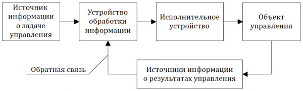
Fig. 1.1.1 — Structure of the control system (CS)

If the control system (CS) has a structural diagram that corresponds to Fig. 1.1.1, and operates without human (operator) involvement, it is called an automated control system (ACS).

If the CS operates with human (operator) involvement, it is called an automated control system.

If the Control ensures a specified law of the object's change over time regardless of management results, such control is done in an open loop, and the control itself is called programmatic control.

Systems operating in an open loop include industrial automata (conveyor lines, rotary lines, etc.), numerical control machines (CNC): see example in Fig. 1.1.2.

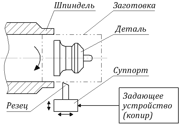
Fig.1.1.2 — Example of programmatic control

The setting device can be, for example, a 'copying device'.

Since this example lacks sensors (measuring devices) to monitor the manufactured part, if, for instance, the tool was improperly set or broke, the set goal (manufacturing the part) cannot be achieved (realized). Typically, output control is necessary in systems of this type to register deviations in dimensions and shape of the part from the desired specifications.

Automatic control systems are divided into 3 types:

automated control systems (ACS);
automatic regulation systems (ARS);
tracking systems (TS).

ARS and TS are subsets of ACS ==> .

Definition: An automatic control system that maintains the constancy of a physical quantity (or group of quantities) in the controlled object is called an automatic control system (ACS).

Automatic control systems (ACS) are the most common type of automatic control systems.

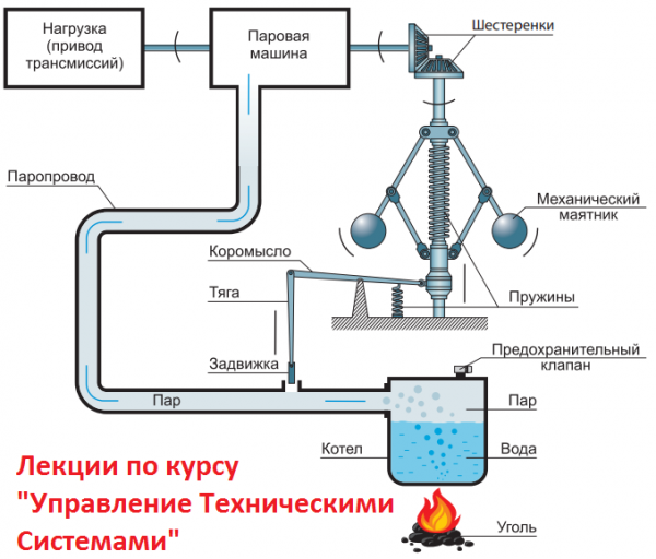
The world's first automatic regulator (18th century) – Watt's regulator. This scheme (see Fig. 1.1.3) was implemented by Watt in England to maintain a constant rotational speed of the steam engine wheel and, consequently, the constant speed of the pulley (belt) of the transmission.

In this scheme, the sensitive elements (measuring sensors) are the "weights" (spheres). The "weights" (spheres) also "actuate" the lever and subsequently the valve. Thus, this system can be classified as a direct control system, and the regulator is a direct action regulator, as it simultaneously serves as both a "measurer" and a "regulator."

In direct action regulators, no additional energy source is required for moving the regulating element.

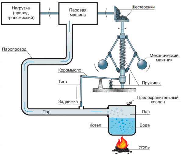
Fig. 1.1.3 – Watt's automatic regulator scheme

In indirect control systems, the presence of an amplifier (for example, power), an additional actuating mechanism containing, for example, an electric motor, servomotor, hydraulic drive, etc., is necessary.

An example of an automatic control system (ACS) in the full sense of this definition could be a control system that ensures a rocket's launch into orbit, where the controlled quantity may be, for example, the angle between the rocket's axis and the normal to Earth ==> see Fig. 1.1.4.a and Fig. 1.1.4.b

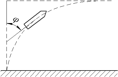
Fig. 1.1.4 (a)

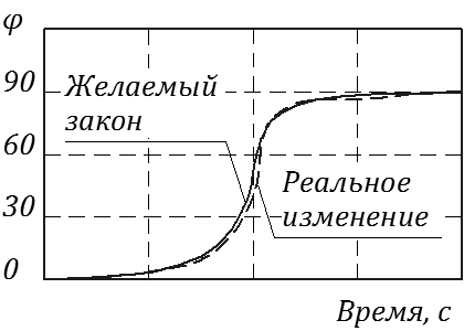
Fig. 1.1.4 (b)

1.2. Structure of control systems: simple and multidimensional systems

In the theory of Control of Technical Systems, any system is traditionally divided into a set of links connected in network structures. In the simplest case, the system contains one link, which receives input influence (input) and produces a system response (output).

In the theory of Control of Technical Systems, there are 2 main ways to represent the links of control systems:

— in terms of "input-output";

— in state variables (see sections 6…7 for more details).

The representation in input-output variables is typically used to describe relatively simple systems, which have one 'input' (one control action) and one 'output' (one controlled quantity, see Figure 1.2.1).

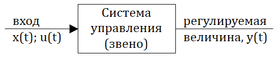
Fig. 1.2.1 – Schematic representation of a simple control system

This description is usually applied to technically simple automated control systems (ACS).

Recently, the representation in state variables has gained widespread use, especially for technically complex systems, including multidimensional ACS. Figure 1.2.2 presents a schematic representation of a multidimensional automated control system, where u1(t)…um(t) — control actions (control vector), y1(t)…yp(t) — controlled parameters of ACS (output vector).

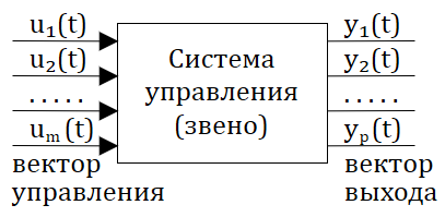
Fig. 1.2.2 — Schematic representation of a multidimensional control system.

Let’s take a closer look at the structure of ACS, presented in input-output variables and having one input (input or setpoint or control action) and one output (output action or controlled (or regulated) variable).

Assume that the structural diagram of such ACS consists of a certain number of elements (links). By grouping the links according to functional principles (what the links do), the structural diagram of ACS can be represented in the following typical form:

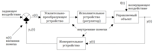
Fig. 1.2.3 — Structural diagram of an automated control system

The symbol ε(t) or the variable ε(t) denotes the mismatch (error) at the output of the comparison device, which can 'operate' in modes of both simple comparative arithmetic operations (most often subtraction, less often addition) as well as more complex comparative operations (procedures).

Since y1(t) = y(t)*k1, where k1 — gain factor, thus ==>
ε(t) = x(t) — y1(t) = x(t) — k1*y(t)

The task of the control system is to 'work' to eliminate the mismatch (error) (if it is stable), ε(t), that is, ==> ε(t) → 0.

It should be noted that both external influences (controlling, disturbing, noise) and internal disturbances affect the control system. A disturbance differs from an influence in that it is stochastic (random) in nature, while an influence is almost always deterministic.

To denote the controlling (input) signal, we will use either x(t), or u(t).

1.3. Basic Laws of Control

If we return to the last figure (the structural diagram of the control system in Fig. 1.2.3), it is necessary to 'decode' the role played by the amplifying-transforming device (what functions it performs).

If the amplifying-transforming device (ATD) performs only amplification (or attenuation) of the mismatch signal ε(t), namely: , where – the proportionality coefficient (in the particular case = Const), then this mode of closed-loop control is called the proportional control (P-control).

If the ATD generates an output signal ε1(t) proportional to the error ε(t) and the integral of ε(t), i.e. , then this mode of control is called proportional-integral (PI-control). ==> , where b – the proportionality coefficient (in the particular case b = Const).

Usually, PI-control is used to improve control (regulation) accuracy.

If the ATD generates an output signal ε1(t) proportional to the error ε(t) and its derivative, then this mode is called proportional-derivative (PD-control): ==>

Usually, the use of PD-control increases the performance of the control system.

If the ATD generates an output signal ε1(t) proportional to the error ε(t), its derivative, and the integral of the error ==> , then this mode of control is called proportional-integral-derivative control (PID-control).

PID-control often allows for 'good' control accuracy with 'good' performance.

1.4. Classification of Automatic Control Systems

1.4.1. Classification by Type of Mathematical Description

By the type of mathematical description (equations of dynamics and statics), automatic control systems (ACS) are classified into linear and nonlinear systems (ACS or APC).

Each "subclass" (linear and nonlinear) is subdivided into several "subclasses." For example, linear automatic control systems (ACS) vary according to the type of mathematical description.
Since this semester will focus on the dynamic properties of only linear automatic control systems (regulation), we will provide a classification based on the type of mathematical description for linear ACS below:

1) Linear automatic control systems described in "input-output" variables by ordinary differential equations (ODE) with constant coefficients:

where x(t) – input effect; y(t) – output effect (controlled variable).

If we use the operator ("compact") form of writing the linear ODE, equation (1.4.1) can be presented as follows:

where, p = d/dt — differentiation operator; L(p), N(p) — corresponding linear differential operators, which are equal to:

2) Linear automatic control systems described by linear ordinary differential equations (ODE) with variable (in time) coefficients:

In general, such systems can also be classified as nonlinear ACS.

3) Linear automatic control systems described by linear difference equations:

where f(…) – linear function of arguments; k = 1, 2, 3… — integers; Δt – quantization interval (discretization interval).

Equation (1.4.4) can be represented in a "compact" form:

Usually, such a description of linear ACS is used in digital control systems (using computers).

4) Linear automatic control systems with delay:

where L(p), N(p) — linear differential operators; τ — delay time or delay constant.

If the operators L(p) and N(p) degenerate (L(p) = 1; N(p) = 1), then equation (1.4.6) corresponds to the mathematical description of the dynamics of a perfect delay element:

and a graphical illustration of its properties is shown in Figure 1.4.1

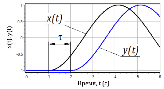
Figure 1.4.1 — Graphs of input and output of the perfect delay element

5) Linear automatic control systems described by linear differential equations in partial derivatives.Such ACS are often referred to as distributed control systems. ==> "Abstract" example of such a description:

The system of equations (1.4.7) describes the dynamics of a linearly distributed automatic control system, i.e., the controlled variable depends not only on time but also on one spatial coordinate.
If the control system is a "spatial" object, then ==>

where it depends on time and spatial coordinates defined by the radius-vector.

6) Automatic control systems described by systems of ordinary differential equations, or systems of difference equations, or systems of partial differential equations ==>, and so forth…

A similar classification can also be proposed for nonlinear automatic control systems (ACS)…

For linear systems, the following requirements are met:

linearity of the static characteristic of the ACS;
linearity of the dynamic equation, i.e., the variables in the dynamic equation enter only in linear combinations.

The static characteristic is defined as the dependence of the output on the magnitude of the input influence in a steady state (when all transients have dissipated).

For systems described by linear ordinary differential equations with constant coefficients, the static characteristic is derived from the dynamic equation (1.4.1) by setting all non-stationary terms to zero ==>

Figure 1.4.2 shows examples of linear and nonlinear static characteristics of automatic control systems.

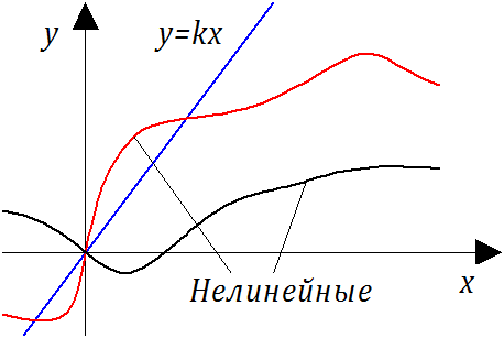
Fig. 1.4.2 — Examples of static linear and nonlinear characteristics

Nonlinearity of the terms containing time derivatives in the dynamic equations may occur when using nonlinear mathematical operations (*, /, , , sin, ln, etc.). For example, considering the dynamic equation of some "abstract" ACS

note that in this equation with a linear static characteristic the second and third terms (dynamic terms) in the left part of the equation — nonlinear, therefore, the ACS described by such an equation is nonlinear in the dynamic plane..

1.4.2. Classification by the nature of the transmitted signals

By the nature of the transmitted signals, automatic control systems (or regulation) are divided into:

continuous systems (continuous action systems);
relay systems (relay action systems);
discrete action systems (impulse and digital systems).

System continuous. the actions are called such control systems, in each of whose elements continuous changes in the input signal over time corresponds to a continuous change of the output signal, while the law of change of the output signal can be arbitrary. For the control system to be continuous, it is necessary for the static characteristics of all elements to be continuous.

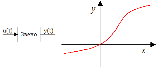
Fig. 1.4.3 — Example of a continuous system

System relay actions is called a control system, in which at least in one element, with continuous change in the input quantity, the output quantity changes 'jumping' at certain moments of the control process depending on the magnitude of the input signal. The static characteristic of such an element has discontinuities or breaks with discontinuities.

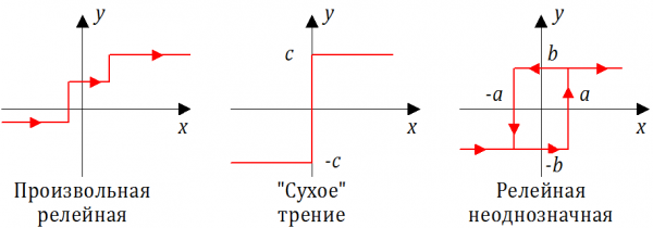
Fig. 1.4.4 — Examples of relay static characteristics

System discrete actions is a system in which at least in one element, with continuous change in the input quantity, the output quantity has the form of individual pulses, appearing after a certain time interval.

An element that converts a continuous signal into a discrete signal is called a pulse element. Such a type of transmitted signals occurs in control systems with a computer or controller.

The following methods (algorithms) for converting a continuous input signal into a pulse output signal are most commonly implemented:

amplitude-pulse modulation (APM);
width-pulse modulation (WPM).

Fig. 1.4.5 presents a graphical illustration of the amplitude-pulse modulation (APM) algorithm. In the upper part of the figure, the time dependence is presented x(t) — of the signal at the input of the pulse element. The output signal of the pulse block (element) y(t) – is a sequence of rectangular pulses appearing with constant a quantization period Δt (see the lower part of the figure). The duration of the pulses is the same and equal to Δ. The amplitude of the pulse at the output of the block is proportional to the corresponding value of the continuous signal x(t) at the input of this block.

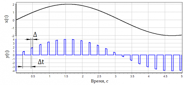
Fig. 1.4.5 — Implementation of amplitude-pulse modulation

This method of pulse modulation was quite common in electronic measuring equipment of control and protection systems in nuclear power plants in the 70s and 80s of the last century.

Figure 1.4.6 presents a graphical illustration of the Pulse Width Modulation (PWM) algorithm. At the top of Fig. 1.14, the time dependence x(t) of the signal at the input of the impulse unit is shown. The output signal of the impulse block y(t) is a sequence of rectangular pulses appearing at a constant quantization period Δt (see the lower part of Fig. 1.14). The amplitude of all pulses is the same. The pulse duration Δt at the output of the block is proportional to the corresponding value of the continuous signal x(t) at the input of the impulse block.

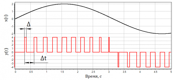
Fig. 1.4.6 — Implementation of Pulse Width Modulation

This method of pulse modulation is currently the most widely used in electronic measuring equipment of control and protection systems (CPS) for nuclear energy installations (NEI) and automated control systems (ACS) of other technical systems.

In conclusion of this subsection, it should be noted that if the characteristic time constants in other sections of the ACS (CPS) are significantly greater than Δt (by orders of magnitude), then the pulse system can be considered as a continuous automatic control system (when using both PWM and PWM).

1.4.3. Classification by Type of Control

By the nature of the control processes, automatic control systems are divided into the following types:

deterministic ACS, where a unique output signal can be assigned to the input signal (and vice versa);
stochastic ACS (statistical, probabilistic), where a given input signal has a random (stochastic) output signal.

The output stochastic signal is characterized by:

the distribution law;
the mathematical expectation (mean value);
the variance (standard deviation).

The stochastic nature of the control process is usually observed in significantly nonlinear ACS both in terms of static characteristics and in terms of (even more so) the nonlinearity of dynamic components in the dynamics equations.

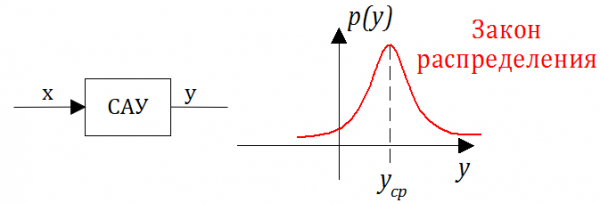
Fig. 1.4.7 — Distribution of the output value of a stochastic ACS

In addition to the main types of classification of control systems, there are other classifications. For example, classification can be based on the method of control and the interaction with the external environment, as well as the ability of automated control systems to adapt to changes in environmental parameters. Systems are divided into two major classes:

1) Ordinary (non-adaptive) control systems without adaptation; these systems are considered simple and do not change their structure during the control process. They are the most developed and widely used. Ordinary control systems are divided into three subclasses: open-loop, closed-loop, and combined control systems.

2) Adaptive control systems. In these systems, when external conditions or characteristics of the regulated object change, there is an automatic (unspecified in advance) change in the parameters of the control device due to changes in the coefficients of the control system, the structure of the control system, or even the introduction of new elements.

Another example of classification is hierarchical classification (single-level, two-level, multi-level).

Only registered users can participate in the survey. Please log in, please.