Hello, Habr! I present to your attention the translation of the article.
"How does a relational database work".

When it comes to relational databases, I can't help but feel something is missing. They are used everywhere. There are many different databases, from the small and handy SQLite to the powerful Teradata. Yet, there are only a few articles that explain how a database works. You can search for yourself with the query "howdoesarelationaldatabasework" to see how few results there are. Moreover, these articles are short. If you're looking for the latest trendy technologies (Big Data, NoSQL, or JavaScript), you'll find more in-depth articles explaining how they work.

Are relational databases too old and too boring to explain outside of university courses, research papers, and books?

As a developer, I hate using what I don't understand. And if databases have been around for over 40 years, there must be a reason. Over the years, I’ve spent hundreds of hours truly understanding these strange black boxes that I use every day. Relational databases are very interesting because they are based on useful and reusable concepts.If you are interested in understanding databases but have never had the time or desire to delve into this vast topic, you should enjoy this article.

Although the title of this article is explicit, the goal of this article is not to understand how to use a database.Therefore, you should already know how to write a simple join query and basic queries; CRUDotherwise, you may not understand this article. That's the only thing you need to know; I'll explain everything else.

I'll start with some basics of computer science, such as the time complexity of algorithms (Big O). I know some of you hate this concept, but without it, you won't be able to grasp the intricacies within a database. Since this is a huge topic, I will focus on what I consider important, how a database processes: queries. SQL queryI will present only the core concepts of databasesso that by the end of the article, you have an understanding of what happens under the hood.

Since this is a lengthy and technical article that includes numerous algorithms and data structures, take your time to read through it. Some concepts may be difficult to grasp; you can skip them and still gain a general understanding.

For those of you who are more informed, this article is divided into three parts:

Overview of low-level and high-level database components
Overview of query optimization processes
Overview of transaction management and buffer pool

Back to basics

Many years ago (in a galaxy far, far away…), developers had to know exactly how many operations they were coding. They memorized their algorithms and data structures because they couldn’t afford to waste the CPU and memory of their slow computers.

In this part, I will remind you of some of these concepts, as they are necessary for understanding databases. I will also introduce the concept of database indexing.

O(1) vs O(n²)

Nowadays, many developers don’t care about the time complexity of algorithms… and they are right!

But when you are dealing with large amounts of data (I’m not talking about thousands) or if you’re fighting for milliseconds, it becomes critically important to understand this concept. And as you can imagine, databases have to handle both situations! I won’t make you spend more time than necessary to grasp the essence. This will help us later understand the concept of cost-based optimization (cost based optimization).

Concept

The time complexity of an algorithm is used to see how long it will take to execute the algorithm for a given amount of data.To describe this complexity, mathematical notations of big O are used. This notation is employed with a function that describes how many operations an algorithm requires for a given amount of input data.

For example, when I say "this algorithm has a complexity of O(some_function())", it means that to process a certain amount of data, the algorithm requires some_function(a_certain_amount_of_data) operations.

At this point, It’s not about the quantity of data,but rather how the number of operations increases as the amount of data grows.Time complexity does not provide an exact number of operations, but it’s a good way to estimate execution time.

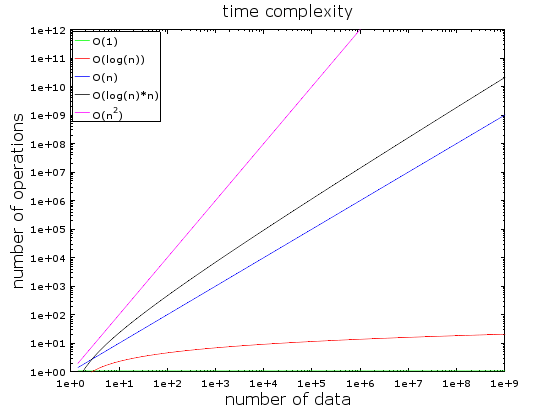
In this graph, you can see the dependency of the number of operations on the volume of input data for various types of algorithm time complexities. I used a logarithmic scale to display them. In other words, the amount of data increases rapidly from 1 to 1 billion. We can see that:

O(1) or constant complexity remains constant (otherwise it would not be called constant complexity).
O(log(n)) remains low even with billions of data.
The worst-case complexity is O(n2), where the number of operations increases rapidly.
The other two complexities also increase quickly.

Examples

With a small amount of data, the difference between O(1) and O(n2) is negligible. For example, suppose you have an algorithm that needs to process 2000 elements.

The O(1) algorithm will cost you 1 operation
The O(log(n)) algorithm will cost you 7 operations
The O(n) algorithm will cost you 2000 operations
The O(n * log(n)) algorithm will cost you 14,000 operations
The O(n2) algorithm will cost you 4,000,000 operations

The difference between O(1) and O(n2) seems large (4 million operations) but you will lose at most 2 ms, just the time it takes to blink. Indeed, modern processors can handle hundreds of millions of operations per second.That’s why performance and optimization are not an issue in many IT projects.

As I mentioned, it is still important to know this concept when working with large amounts of data. This time, if the algorithm needs to process 1,000,000 elements (which is not that much for a database):

The O(1) algorithm will cost you 1 operation
The O(log(n)) algorithm will cost you 14 operations
The O(n) algorithm will cost you 1,000,000 operations
The O(n * log(n)) algorithm will cost you 14,000,000 operations
The O(n2) algorithm will cost you 1,000,000,000,000 operations

I didn’t do the calculations, but I would say that with an O(n2) algorithm, you have time to grab a coffee (even two!). If you add another 0 to the data volume, you’ll have time for a nap.

Let’s dive deeper

For reference:

Searching in a good hash table finds an element in O(1).
Searching in a well-balanced tree gives a result in O(log(n)).
Searching in an array gives a result in O(n).
The best sorting algorithms have a complexity of O(n * log(n)).
A poor sorting algorithm has a complexity of O(n2).

Note: In the following sections, we will see these algorithms and data structures.

There are several types of algorithm time complexity:

average case scenario
best case scenario
and worst case scenario

Time complexity is often considered the worst case scenario.

I only talked about the time complexity of an algorithm, but complexity also applies to:

memory consumption by the algorithm
disk I/O consumption by the algorithm

Of course, there are complexities worse than n2, such as:

n4: that's terrible! Some of the mentioned algorithms have this complexity.
3n: that’s even worse! One of the algorithms we will see in the middle of this article has this complexity (and it is indeed used in many databases).
factorial n: you will never get your results even with a small amount of data.
nn: if you encounter this complexity, you should ask yourself if this is really your area of expertise…

Note: I have given you not a real definition of the "big O" notation, but just an idea. You can read this article for a real (asymptotic) definition. Wikipedia for a real (asymptotic) definition.

MergeSort

What do you do when you need to sort a collection? What? You call the sort() function… Ok, good answer… But for databases, you need to understand how the sort() function works.

There are several good sorting algorithms, so I will focus on the most important one: merge sort. You may not understand now why sorting data is useful, but you will after the section dedicated to query optimization. Moreover, understanding merge sort will help us later understand a common database operation called merge join merge join.

Merge

Like many useful algorithms, merge sort is based on a trick: merging 2 sorted arrays of size N/2 into an N-element sorted array takes only N operations. This operation is called merging.

Let’s see what this means with a simple example:

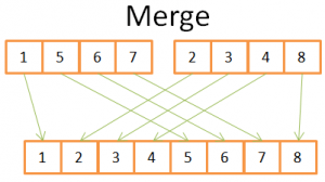
In this illustration, you can see that to build the final sorted array of 8 elements, you only need to iterate once through 2 4-element arrays. Since both 4-element arrays are already sorted:

1) you compare both current elements in the two arrays (at the beginning current = first)
2) then take the smallest one to place it in an array of 8 elements
3) and move to the next element in the array where you took the smallest element
and repeat 1, 2, 3 until you reach the last element of one of the arrays.
Then you take the remaining elements from the other array to place them in an array of 8 elements.

This works because both 4-element arrays are sorted, so you don't need to 'go back' in these arrays.

Now that we understand this trick, here's my pseudocode for merge:

array mergeSort(array a)
   if(length(a)==1)
      return a[0];
   end if

   //recursive calls
   [left_array right_array] := split_into_2_equally_sized_arrays(a);
   array new_left_array := mergeSort(left_array);
   array new_right_array := mergeSort(right_array);

   //merging the 2 small ordered arrays into a big one
   array result := merge(new_left_array,new_right_array);
   return result;

Merge sort divides the task into smaller tasks, then finds the results of the smaller tasks to obtain the result of the original task (note: this kind of algorithm is called divide and conquer). If you don't understand this algorithm, don't worry; I didn't get it the first time I saw it. If it helps, I see this algorithm as a two-phase algorithm:

Division phase, where the array is divided into smaller arrays
Sorting phase, where the small arrays are combined (using merging) to form a larger array.

Division phase

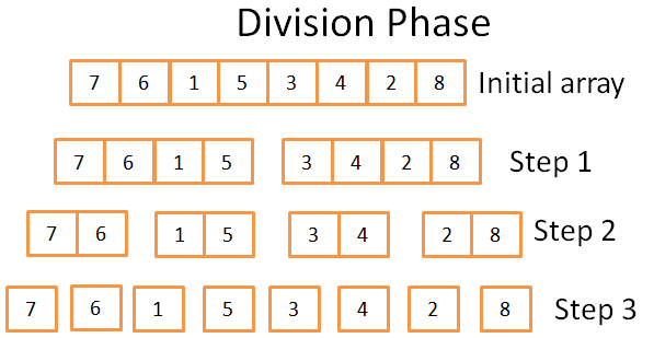
During the division phase, the array is divided into unitary arrays in 3 steps. The formal number of steps is log(N) (since N=8, log(N) = 3).

How do I know this?

I'm a genius! In a word — math. The idea is that each step divides the size of the original array by 2. The number of steps is how many times you can divide the original array into two. This is the precise definition of a logarithm (base 2).

Sorting phase

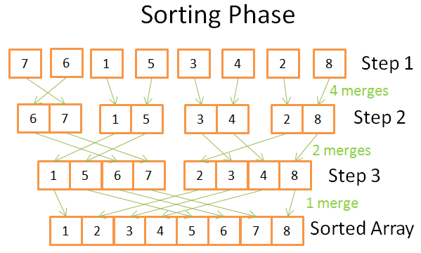
During the sorting phase, you start with unitary (one-element) arrays. At each stage, you perform several merge operations, and the total cost is N = 8 operations:

At the first stage, you have 4 merges costing 2 operations each
At the second step, you have 2 merges costing 4 operations each
At the third step, you have 1 merge costing 8 operations

Since there are log(N) steps, the total cost N * log(N) operations.

Advantages of merge sort

Why is this algorithm so powerful?

Because:

You can modify it to reduce memory usage, so that you do not create new arrays but directly modify the input array.

Note: this type of algorithm is called in—place (sorting without additional memory).

You can modify it to use disk space simultaneously while keeping memory usage low without significant I/O costs. The idea is to load into memory only the parts that are currently being processed. This is important when you need to sort a table that is several gigabytes in size with only a 100 megabyte memory buffer.

Note: this type of algorithm is called external sorting.

You can modify it to run on multiple processes/threads/servers.

For example, distributed merge sort is one of the key components : depends on you (which is a structure in big data).

This algorithm can turn lead into gold (really!).

This sorting algorithm is used in most (if not all) databases, but it is not the only one. If you want to learn more, you can read this research paper, which discusses the pros and cons of common sorting algorithms in databases.

Array, Tree, and Hash Table

Now that we understand the idea of time complexity and sorting, I need to tell you about three data structures. This is important because they are the foundation of modern databases.. I will also introduce the concept of database indexing.

Array

A two-dimensional array is the simplest data structure. A table can be viewed as an array. For example:

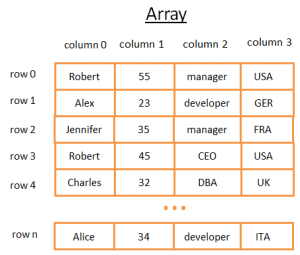
This 2D array represents a table with rows and columns:

Each row represents an entity.
Columns store properties describing the entity.
Each column stores data of a specific type (integer, string, date, etc.).

This makes it convenient to store and visualize data; however, when you need to find a specific value, it is not suitable.

For example, if you want to find all the guys who work in the UK, you will need to check each row to determine if that row belongs to the UK. This will cost you N operations., where N — the number of rows, which isn't bad, but could there be a faster way? Now it’s time to get acquainted with trees.

Note: most modern databases provide extended arrays for efficient storage of tables: heap-organized tables and index-organized tables. However, this doesn't change the problem of quickly searching for a specific condition in a group of columns.

Database Tree and Index

A binary search tree is a binary tree with a special property: the key in each node must be:

greater than all keys stored in the left subtree
less than all keys stored in the right subtree

Let's see what this means visually

Idea

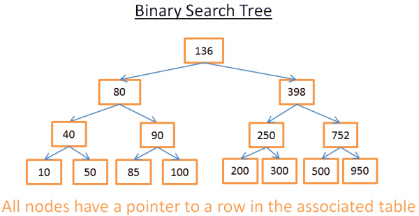
This tree has N = 15 elements. Suppose I am looking for 208:

I start at the root, whose key is 136. Since 136 < 208, I look at the right subtree of node 136.
398 > 208, therefore, I look at the left subtree of node 398
250 > 208, therefore, I look at the left subtree of node 250
200 < 208, therefore, I look at the right subtree of node 200. But 200 does not have a right subtree, the value does not exist (because if it existed, it would be in the right subtree of 200).

Now, let's say I am looking for 40

I start at the root, whose key is 136. Since 136 > 40, I look at the left subtree of node 136.
80 > 40, therefore, I look at the left subtree of node 80
40= 40, the node exists. I extract the row ID within the node (this is not shown in the picture) and look up the table for the given row ID.
Knowing the row ID allows me to know exactly where the data is located in the table, and therefore I can retrieve it instantly.

In the end, both searches will cost me the number of levels within the tree. If you read the part about merge sorting carefully, you should see that there are log(N) levels here. Therefore, the cost of search is log(N), not bad!

Let's return to our problem

But this is very abstract, so let's get back to our problem. Instead of a simple integer, imagine a string representing someone's country in the previous table. Suppose you have a tree that contains a "country" field (column 3) of the table:

If you want to know who works in the UK
you look at the tree to get the node that represents the UK
inside the "UK node" you will find the location of employee records in the UK.

This search will cost log(N) operations instead of N operations if you directly use an array. What you just presented was a database index.

You can build an index tree for any group of fields (string, number, 2 strings, number and string, date...) as long as you have a function to compare keys (i.e., groups of fields) so that you can establish the order among keys (which holds for any basic types in the database).

B+TreeIndex

Although this tree works well for retrieving a specific value, there is a BIG problem when you need to retrieve multiple items between two values. It will cost O(N) because you will have to look at each node in the tree and check if it lies between those two values (for example, with an in-order traversal of the tree). Moreover, this operation is not convenient for disk I/O, as you will need to read the entire tree. We need to find a way to efficiently execute a range query. To address this problem, modern databases use a modified version of the previous tree called B+Tree. In a B+Tree:

only the lowest nodes (leaves) store the information (location of rows in the related table)
the other nodes are here to route to the correct node during a search.

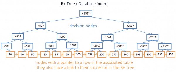
As you can see, there are more nodes here (twice as many). Indeed, you have additional nodes, 'decision nodes,' which help you find the correct node (which stores the location of rows in the related table). However, the search complexity is still O(log(N)) (there is just one more level). The big difference is that the nodes at the lower level are connected to their successors.

With this B+Tree, if you are searching for values from 40 to 100:

You just need to search for 40 (or the nearest value after 40 if 40 does not exist), as you did with the previous tree.
Then, gather the successors of 40 using direct links to the successors until you reach 100.

Assuming you found M successors, and the tree has N nodes. Searching for a specific node costs log(N) similar to the previous tree. But, having found this node, you will retrieve M successors in M operations with links to their successors. This search only costs M+log(N) operations compared to N operations with the previous tree. Moreover, you don't have to read the entire tree (only M + log(N) nodes), which means less disk usage. If M is small (e.g., 200 rows) and N is large (1,000,000 rows), this will make a BIG difference.

But here come new issues (again!). If you add or delete a row in the database (and thus in the associated B+Tree index):

you must maintain the order among the nodes within the B+Tree; otherwise, you won't be able to find nodes within an unsorted tree.
you need to keep the number of levels in the B+Tree as low as possible; otherwise, the time complexity from O(log(N)) will become O(N).

In other words, the B+Tree must be self-ordering and balanced. Fortunately, this is achievable with smart deletion and insertion operations. But it comes at a high cost: insertion and deletion in a B+Tree cost O(log(N)). That’s why some of you may have heard that using too many indexes is not a very good idea. Indeed, you slow down the quick insertion/update/deletion of a row in the table, as the database needs to update the table's indexes with a costly O(log(N)) operation for each index. Moreover, adding indexes means more load on the transaction manager (to be described at the end of the article).

For more detailed information, you can check the Wikipedia article on B+Tree. If you want an example of a B+Tree implementation in a database, take a look this article and this article from the leading MySQL developer. They both focus on how InnoDB (the MySQL engine) handles indexes.

Note: a reader told me that due to low-level optimizations, the B+Tree must be fully balanced.

Hashtable

Our last important data structure is the hash table. It's very useful when you want to quickly look up values. Moreover, understanding hash tables will help us later grasp a common database operation called hash join ( hash join). This data structure is also used by the database to store some internal things (e.g., lock table or buffer pool, we will see both of these concepts later).

A hash table is a data structure that quickly finds an element by its key. To build a hash table, you need to define:

the key for your elements
the hash function for the keys. The computed hashes of the keys provide the locations of the elements (called segments ).
a function for comparing keys). Once you've found the right segment, you must find the element you are looking for within the segment using this comparison.

A simple example

Let's take a practical example:

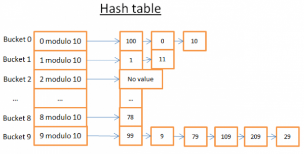
This hash table has 10 segments. Since I'm lazy, I've depicted only 5 segments, but I know you are smart, so I'll let you imagine the other 5 yourself. I used a hash function based on the modulo 10 of the key. In other words, I keep only the last digit of the element's key to find its segment:

if the last digit is 0, the element goes into segment 0,
if the last digit is 1, the element goes into segment 1,
if the last digit is 2, the element goes into segment 2,
…

The comparison function I used is simply equality between two integers.

Let's say you want to retrieve the element 78:

The hash table computes the hash code for 78, which equals 8.
The hash table looks in segment 8, and the first element it finds is 78.
It returns the element 78 to you
The search costs only 2 operations (one for computing the hash function value and the other for finding the element within the segment).

Now, let's say you want to retrieve the element 59:

The hash table computes the hash code for 59, which equals 9.
The hash table searches in segment 9; the first found element is 99. Since 99 != 59, the element 99 is not the correct element.
Using the same logic, it takes the second element (9), the third (79), …, the last (29).
Element not found.
The search cost was 7 operations.

A good hash function

As you can see, depending on the value you are searching for, the cost is not the same!

If I now change the hash function to modulo 1,000,000 of the key (that is, taking the last 6 digits), the second search would cost only 1 operation, since there are no elements in segment 000059. The real challenge is to find a good hash function that creates segments containing very few elements..

In my example, finding a good hash function is easy. But this is a simple example; finding a good hash function is more challenging when the key is:

a string (e.g., last name)
2 strings (e.g., last name and first name)
2 strings and a date (e.g., last name, first name, and birth date)
…

With a good hash function, searching in a hash table takes O(1).

Array vs Hash Table

Why not use an array?

Hmm, good question.

A hash table can be partially loaded into memory, while the remaining segments can stay on disk.
With an array, you must use continuous space in memory. If you load a large table, it is very difficult to find enough continuous space..
For a hash table, you can select the desired key (for example, a person's country and last name).

For additional information, you can read the article on Java.HashMap, which is an efficient implementation of a hash table; you do not need to understand Java to grasp the concepts outlined in this article.

Source: habr.com