

Hello Habr.
Many people buying clocks or weather stations might have noticed the Radio Controlled Clock or even Atomic Clock logo on the packaging. It's quite convenient, as you just place the clock on the table, and it will automatically set itself to the correct time after a while.
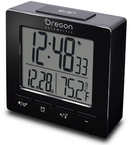
Let's figure out how this works and write a decoder in Python.
There are different time synchronization systems. The most popular one in Europe is the German system , in Japan, there is its own system , in the USA, there is a system , and so on. The following discussion will be about DCF77, as it's the most relevant and accessible for reception in some areas of the European part of Russia and neighboring countries (residents of the Far East might have a different opinion, but they can, in turn, receive and analyze the Japanese signal;).
Everything written below will be about DCF77.
Receiving the signal
DCF77 is a long-wave station operating at a frequency of 77.5 kHz, transmitting signals in amplitude modulation. The station, with a power of 50 kW, is located 25 km from Frankfurt; it started operations back in 1959, and in 1973, date information was added to the precise time. The wavelength at a frequency of 77 kHz is quite large, so the size of the antenna field is also quite significant (photo from Wikipedia):
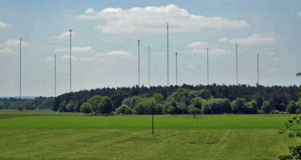
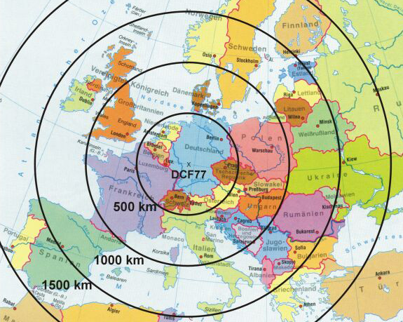
With such an antenna and applied power, the reception area covers almost all of Europe, Belarus, Ukraine, and parts of Russia.
Anyone can record the signal. To do this, just go to the online receiver , select the frequency of 76.5 kHz and USB modulation. An image similar to the following should open:
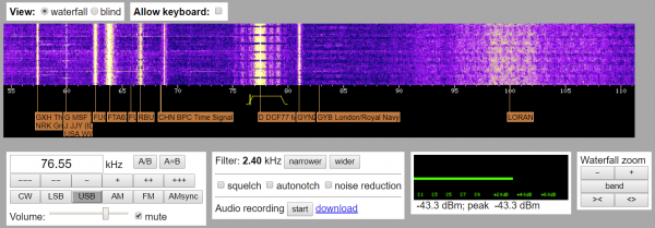
There, click the download button and record a segment lasting several minutes. Of course, if you have a 'real' receiver capable of capturing the 77.5 kHz frequency, you can use it as well.
Of course, receiving precise time radio signals over the Internet won't give us truly accurate time — the signal is transmitted with a delay. But our goal is just to understand the signal structure, and for that, internet recordings are more than enough. In reality, specialized devices for receiving and decoding are used, and these will be discussed below.
So, we have obtained the recording; let's proceed with its processing.
Decoding the signal
We'll load the file using Python and take a look at its structure:
from scipy.io import wavfile
from scipy import signal
import matplotlib.pyplot as plt
import numpy as np

sample_rate, data = wavfile.read("dcf_websdr_2019-03-26T20_25_34Z_76.6kHz.wav")
plt.plot(data[:100000])
plt.show()
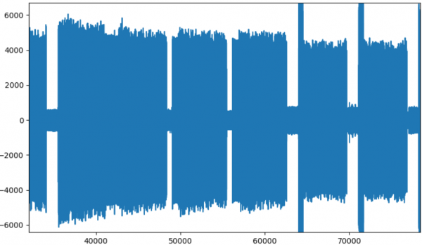
We see typical amplitude modulation:
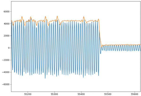
To simplify the decoding, let's take the signal's envelope using the Hilbert transform:
analytic_signal = signal.hilbert(data)
A = np.abs(analytic_signal)
plt.plot(A[:100000])
The result shown in an enlarged view:
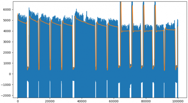
We will smooth out noise by using a low-pass filter and calculate the average value, which will be useful for parsing later.
b, a = signal.butter(2, 20.0/sample_rate)
zi = signal.lfilter_zi(b, a)
A, _ = signal.lfilter(b, a, A, zi=zi*A[0])
avg = (np.amax(A) + np.amin(A))/2
The result (yellow line): a nearly rectangular signal that is quite easy to analyze.
Parsing
First, we need to obtain the bit sequence. The structure of the signal is very simple.
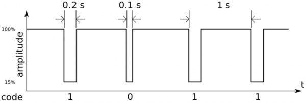
The impulses are divided into one-second intervals. If the distance between impulses is 0.1s (i.e., the impulse duration is 0.9s), we add '0' to the bit sequence; if the distance is 0.2s (i.e., duration is 0.8s), we add '1'. The end of each minute is marked by a 'long' impulse lasting 2s, during which the bit sequence resets and starts anew.
The above can easily be coded in Python.
sig_start, sig_stop = 0, 0
pos = 0
bits_str = ""
while pos < cnt - 4:
    if A[pos]  avg:
        # Signal begin
        sig_start = pos
    if A[pos] > avg and A[pos+1] < avg:
        # Signal end
        sig_stop = pos

        diff = sig_stop - sig_start

        if diff  0.85*sample_rate and diff  1.5*sample_rate:
            print(bits_str)
            bits_str = ""

    pos += 1
As a result, we obtain a sequence of bits; in our example, for two seconds, it looks like this:
0011110110111000001011000001010000100110010101100010011000
 0001111100110110001010100001010000100110010101100010011000
Interestingly, there is also a 'second layer' of data in the signal. The sequence of bits is also encoded using . Theoretically, this should ensure more robust decoding even in the case of a weakened signal.
Our final step: to obtain the actual data. The bits are transmitted once per second, giving us a total of 59 bits, which contain quite a bit of information:
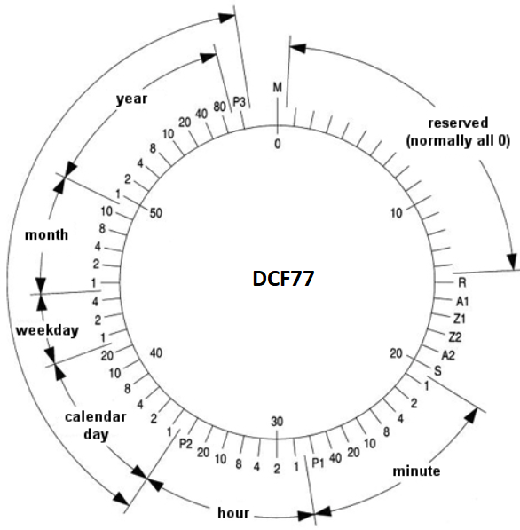
The bits are described in , and they are quite curious. The first 15 bits are not used, although there were plans to use them for alert systems and civil defense. Bit A1 indicates that the clocks will be set forward for daylight saving time in the next hour. Bit A2 indicates that an additional , which is sometimes used to adjust time according to the Earth's rotation. The remaining bits encode hours, minutes, seconds, and date.
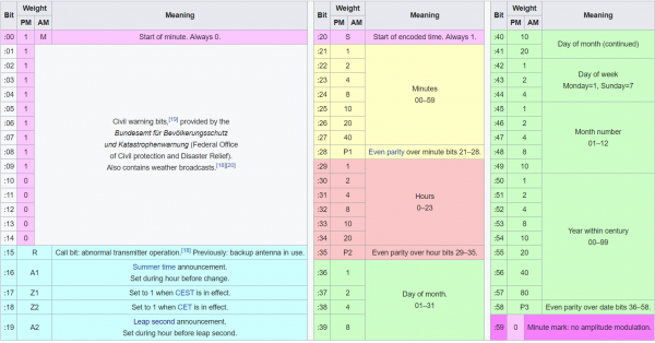
For those who would like to experiment on their own, the decoding code is provided in the spoiler below.
Source Code
def decode(bits):
    if bits[0] != '0' or bits[20] != '1':
        return

    minutes, hours, day_of_month, weekday, month, year = map(convert_block,
                                                             (bits[21:28], bits[29:35], bits[36:42], bits[42:45],
                                                              bits[45:50], bits[50:58]))
    days = ('Sunday', 'Monday', 'Tuesday', 'Wednesday', 'Thursday', 'Friday', 'Saturday', 'Sunday')
    print('{dow}, {dom:02}.{mon:02}.{y}, {h:02}:{m:02}'.format(h=hours, m=minutes, dow=days[weekday],
                                                               dom=day_of_month, mon=month, y=year))


def convert_ones(bits):
    return sum(2**i for i, bit in enumerate(bits) if bit == '1')


def convert_tens(bits):
    return 10*convert_ones(bits)


def right_parity(bits, parity_bit):
    num_of_ones = sum(int(bit) for bit in bits)
    return num_of_ones % 2 == int(parity_bit)


def convert_block(bits, parity=False):
    if parity and not right_parity(bits[:-1], bits[-1]):
        return -1

    ones = bits[:4]
    tens = bits[4:]
    return convert_tens(tens) + convert_ones(ones)
By running the program, we will see output similar to this:
0011110110111000001011000001010000100110010101100010011000
 Tuesday, 03/26/19, 21:41
 0001111100110110001010100001010000100110010101100010011000
 Tuesday, 03/26/19, 21:42
So that's all the magic. The advantage of this system is that decoding is extremely simple and can be done on any basic microcontroller. We just count the pulse length, accumulate 60 bits, and at the end of each minute, we get the exact time. Compared to other time synchronization methods (like GPS or, heaven forbid, the Internet :), such radio synchronization requires almost no power — for example, a regular home weather station works for about a year on 2 AA batteries. That's why even wristwatches are equipped with radio synchronization, not to mention wall clocks or street station clocks.
The convenience and simplicity of DCF are appealing to DIY enthusiasts. For just $10-20, you can buy a ready-made module with an antenna and a TTL output, which can be connected to an Arduino or another controller.
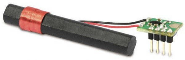
Libraries have already been written for Arduino, and However, it's well-known that whatever you do with a microcontroller results in either a clock or a weather station. With such a device, obtaining accurate time is indeed easy, provided you're within reception range. And you can also attach a label saying 'Atomic Clock' to it, explaining to anyone interested that the device is synchronized using atomic clocks.
Those interested can even upgrade their grandmother's old clock by installing a new radio-synchronized mechanism inside it:
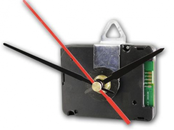
You can find one on eBay using the keywords 'Radio Controlled Movement'.
Finally, a life hack for those who made it this far. Even if there isn't a single radio signal transmitter within a couple thousand kilometers, you can easily generate such a signal yourself. There’s an app on Google Play called 'DCF77 Emulator' that outputs a signal to headphones. According to the author, if you wrap the headphone wire around the clock, it will pick up the signal (interesting how, because regular headphones won't emit a 77kHz signal, but reception likely occurs via harmonics). On my Android 9, the app didn't work at all — there was simply no sound (or maybe I just couldn't hear it — after all, it’s 77kHz :), but maybe someone else will have more luck. Some even build a full DCF signal generator, which is quite easy to create with the same Arduino or ESP32.
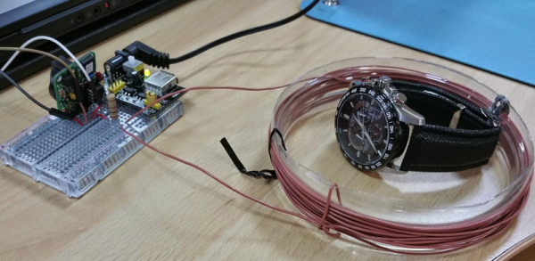
(source )
Conclusion
The DCF system turned out to be quite simple and convenient. With an inexpensive and uncomplicated receiver, you can have accurate time anywhere, of course, within reception range. I believe that even despite the widespread digitalization and the 'internet of things', such simple solutions will remain in demand for a long time.
Source: habr.com
