

In this article, we will discuss how we addressed the issue of a shortage of available storage cells and the development of a discrete optimization algorithm to solve such a problem. We will explain how we 'constructed' a mathematical model for the optimization task and the unexpected difficulties we encountered when processing the input data for the algorithm.
If you are interested in the applications of mathematics in business and are not afraid of applying equivalent transformations of formulas at a 5th-grade level, then welcome under the fold!
This article will be useful for those who implement WMS-systems, work in the field of warehouse or production logistics, as well as programmers interested in the applications of mathematics in business and process optimization within the company.
Introductory Part
This publication continues a series of articles in which we share our successful experience with the implementation of optimization algorithms in warehouse processes.
In We describe the specifics of the warehouse where we implemented the WMS-system, and we also discuss why we needed to solve the problem of clustering batches of remaining goods during the implementation of the WMS-system, and how we approached it.
When we finished writing the article on optimization algorithms, it turned out to be very extensive, so we decided to divide the accumulated material into two parts:
- In the first part (this article), we will describe how we 'constructed' the mathematical model of the problem and the significant challenges we unexpectedly faced when processing and transforming the input data for the algorithm.
- In the second part, we will thoroughly examine the implementation of the algorithm in the C++, conduct a computational experiment, and summarize the experiences we gained during the implementation of such 'intelligent technologies' into the customer's business processes.
How to read the article. If you have read the previous article, you can proceed directly to the chapter 'Overview of Existing Solutions'; if not, the description of the problem being solved is in the spoiler below.
Description of the problem being solved in the customer's warehouse
The bottleneck in the processes
In 2018, we completed a project for the implementation of the WMS-system in the warehouse of 'Trade House LD' in Chelyabinsk. We deployed the product '1C-Logistics: Warehouse Management 3' at 20 workstations: operators WMS, warehouse workers, forklift drivers. The warehouse is medium-sized, about 4,000 m2, with 5,000 cells and 4,500 SKUs. The warehouse stores ball valves of our own production in various sizes from 1 kg to 400 kg. Inventory is stored by batches, as there is a need for goods selection by FIFO.
During the design of automation schemes for warehouse processes, we encountered an existing problem of suboptimal inventory storage. The specifics of storing and stacking valves are such that only the nomenclature of one batch can be located in a cell for individual storage (see Fig. 1). Products arrive at the warehouse daily, and each arrival is a separate batch. In total, after one month of warehouse operation, 30 separate batches are created, and each must be stored in a separate cell. Goods are often selected not by entire pallets, but by individual pieces, resulting in many cells in the individual selection area showing the following situation: in a cell with a volume of over 1m3, there are several pieces of valves occupying less than 5-10% of the cell's volume.
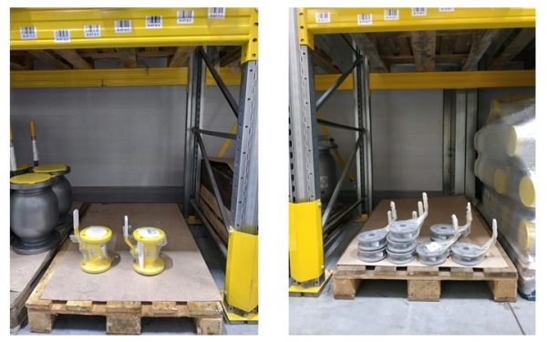
Fig. 1. Photo of several pieces in a cell
There is evident suboptimal use of warehouse capacity. To illustrate the scale of the issue, I can provide numbers: on average, there are between 100 to 300 cells with a volume of over 1m3 containing 'minimal' leftovers at different periods of warehouse operation. Since the warehouse is relatively small, during peak seasons, this factor becomes a 'bottleneck' that significantly slows down the warehouse processes of receiving and shipping.
The idea for solving the problem
The idea arose: to consolidate batches of leftovers with the closest dates into a single batch and to compactly place such leftovers with a unified batch in one cell, or in several if one is not sufficient to accommodate the total amount of leftovers. An example of such 'compression' is shown in Figure 2.
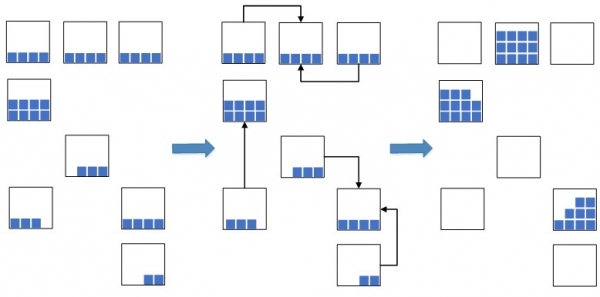
Fig. 2. Scheme for compressing leftovers in cells
This significantly reduces the warehouse space occupied, which will be used for the new goods being stored. In situations with overloaded warehouse capacities, this measure is crucial; otherwise, there may simply not be enough free space to store new items, leading to a halt in the warehouse processes of placement and replenishment and, consequently, a stoppage in receiving and shipping. Previously, before the implementation of the WMS system, this operation was performed manually, which was inefficient since the process of finding suitable stocks in the bins took quite a long time. Now, with the implementation of the WMS system, we have decided to automate, speed up, and make the process intelligent.
The process of solving such a task is divided into 2 stages:
- in the first stage, we find groups of batches that are close in date for compression (this task is dedicated) );
- in the second stage, we calculate the most compact placement of inventory in the bins for each batch group.
In this article, we will focus on the second stage of the algorithm.
Overview of Existing Solutions
Before moving on to the description of the algorithms we developed, it is worth conducting a brief overview of the systems already available on the market WMS, which implement similar functionality for optimal compression.
First of all, it is necessary to note the product "1C: Enterprise 8. WMS Logistics. Warehouse Management 4," which belongs to and is distributed by the company 1C and belongs to the fourth generation WMS-systems developed by AXELOT. This system claims functionality for compression, designed to consolidate fragmented inventory into a single common bin. It should be noted that the compression functionality in such a system also includes other capabilities, such as correcting the placement of items in the bins according to their ABC classes, but we will not dwell on them.
Analyzing the code of the "1C: Enterprise 8. WMS Logistics. Warehouse Management 4" system (which is open in this part of the functionality), we can conclude the following. The algorithm for compressing stocks implements a rather primitive linear logic, and there can be no talk of any 'optimal' compression. Naturally, it does not provide for the clustering of batches. Several clients who have implemented such a system complained about the results of the compression planning. For example, it often happened in practice that when compressing, there was a situation where 100 units of stock from one cell were planned to be moved to another cell, where there was 1 unit of product, although it would be optimal in terms of time to do the opposite.
The functionality for compressing stock in cells is also stated in many foreign WMS-systems, but unfortunately, we have neither real feedback on the effectiveness of the algorithms (this is a trade secret), nor any idea of the depth of their logic (proprietary software with closed code), so we cannot judge.
Searching for a mathematical model of the problem
In order to design quality algorithms to solve the problem, it is necessary first to clearly formulate this problem mathematically, which we will do.
There are many cells  , in which there are stocks of a certain product. We will refer to such cells as donor cells. Let's denote
  the volume of the product located in the cell
  $.
$.
It is important to mention that the compression procedure can involve only one product from one batch, or several batches, which have been preliminarily combined into a cluster (read ), which is due to the specifics of storing and laying out products. Separate compression procedures should be launched for different products or different clusters of batches.
There are many cells  , into which stocks from donor cells can potentially be placed. We will refer to such cells as container cells. These can be either free cells in the warehouse or donor cells from the multitude
  . The multitude is always a subset of
  For each cell
  .
.
from the multitude  there are capacity constraints assigned
  .
.  , measured in dm3. One dm3 represents a cube with sides of 10 cm. The products stored in the warehouse are large enough, so this level of discretization is sufficient in this case.
The matrix of shortest distances is given  in meters between each pair of cells
  , where
  and
and  belong to sets
  and
and  respectively.
Let’s denote  the 'costs' for moving goods from a cell
 to another cell
  . Let’s denote
  the 'costs' for selecting a container
  to move leftovers from other cells into it. How and in what units the values will be calculated
  and
and  will be discussed later (see the section on preparing input data); for now, it's sufficient to say that these quantities will be directly proportional to the amounts
  and
and  respectively.
Let’s denote by  a variable that takes the value 1 if leftovers from a cell
  are moved to a container
  , and 0 otherwise. Let’s denote by
  a variable that takes the value 1 if the container
  contains leftovers, and 0 otherwise.
The problem is formulated as follows: we need to find such a set of containers  and thus 'attach' donor cells to container cells in a way that minimizes the function

under the constraints

Thus, in solving the problem, we aim to:
- firstly, save warehouse capacity;
- secondly, save the time of warehouse workers.
The last constraint means that we cannot move goods to a container that we did not select, and thus did not incur 'costs' for its selection. This constraint also means that the volume of goods moved from cells to the container must not exceed the container's capacity. By the solution of the problem, we mean the set of containers  and the ways of attaching donor cells to containers.
This formulation of the optimization problem is not new and has been studied by many mathematicians since the early 1980s. In foreign literature, there are 2 optimization problems with an appropriate mathematical model: and (we will talk about the differences in tasks later). It is worth mentioning that in mathematical literature, the formulation of these two optimization problems is presented in terms of facility location, hence the name 'Facility Location.' This is largely a matter of tradition, as the need to solve such combinatorial problems first arose from the logistics field, primarily in the military-industrial sector in the 1950s. In terms of facility placement, these problems are formulated as follows:
- There is a finite set of cities where production facilities can potentially be located (hereafter referred to as producer cities). For each producer city, there are specified opening costs for establishing a facility, as well as constraints on the production capacities of the established facility.
- There is a finite set of cities where customers are actually located (hereafter referred to as customer cities). For each customer city, the demand for products is specified. For simplicity, let's consider that the product produced by the facilities and consumed by the customers is the same.
- For each pair of producer city and customer city, there is a specified amount of transportation costs for delivering the required volume of products from the producer to the customer.
It is required to determine in which cities to open facilities and how to assign customers to these facilities so that:
- The total opening costs of the facilities and transportation costs are minimized;
- The demand volume of customers assigned to any open facility does not exceed the production capacities of that facility.
Now it is worth mentioning the only difference between these two classical problems:
- Single-Source Capacitated Facility Location Problem – the customer is supplied only from one open facility;
- Multi-Source Capacitated Facility Location Problem – the customer can be supplied from several open facilities simultaneously.
This difference between the two problems may seem minor at first glance, but in reality, it leads to completely different combinatorial structures of such problems and, consequently, completely different algorithms for solving them. The distinction between the problems is demonstrated in the figure below.
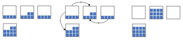
Fig. 3. a) Multi-Source Capacitated Facility Location Problem

Fig. 3. b) Single-Source Capacitated Facility Location Problem
Both problems  -difficult, meaning there is no exact algorithm that can solve such a task in polynomial time based on the input size. In simpler terms, all exact algorithms for solving the task will work in exponential time, although possibly faster than a brute force approach. Since the task
  -is difficult, we will consider only approximate heuristics, meaning algorithms that will compute solutions very close to optimal and will operate quickly enough. If there is interest in such tasks, a good overview can be found here in Russian.
If we relate this to the terminology of our optimal product packing task in cells, then:
- client cities are donor cells
 with product residues,
 - producer cities are container cells , into which residues from other cells are expected to be placed,
- transport costs are time costs for the warehouse worker moving the volume of product from the donor cell to the container cell ;
- opening enterprise costs are the costs of selecting a container , equal to the volume of the container cell , multiplied by some coefficient of saving free volumes (the coefficient value is always > 1) (see section preparing the input data).
 with product residues,
  , into which residues from other cells are expected to be placed,
 for the warehouse worker moving the volume of product from the donor cell
  to the container cell
  ;
;  , equal to the volume of the container cell
  , multiplied by some coefficient of saving free volumes (the coefficient value is always > 1) (see section preparing the input data).
Once the analogy with well-known classic supply problems is established, it is necessary to answer an important question that influences the choice of solution algorithm architecture: is the transfer of residues from the donor cell possible only to one and only one container (Single-Source), or is the transfer possible to multiple container cells (Multi-Source)?
It should be noted that in practice both formulations of the task are present. Below, we present all the 'pros' and 'cons' for each formulation:
| Task option | Pros of the option | Cons of the option |
|---|---|---|
| Single-Source | Goods movement operations calculated according to this task option:
| |
| Multi-Source | Compressing, calculated for this task option, is usually more compact by 10-15% compared to compressions calculated for the 'Single-Source' option. However, it should also be noted that the fewer the stock quantities in the donor cells, the less pronounced this difference in compactness becomes. | Goods movement operations calculated according to this task option:
|
Table 1. Pros and Cons of Single-Source and Multi-Source Options.
Since the number of advantages for the Single-Source option is greater, and considering that the fewer the stock quantities in the donor cells, the smaller the difference in the degree of compactness of compression calculated for both task options, our choice fell on the Single-Source option.
It is worth mentioning that the Multi-Source option also has its place. There are many effective algorithms for solving it, most of which can be reduced to solving a series of transportation problems. There are not only effective algorithms but also elegant ones, for example,
Preparation of Input Data
Before starting the analysis and development of the algorithm for solving the task, it is necessary to determine what data and in what form we will provide it as input. There are no issues with the volumes of goods left in the donor cells and the capacity of the container cells, as this is trivial — such quantities will be measured in m³, but the costs associated with using the container cell and the cost matrix for movement are not so straightforward!
First, let's consider the calculation costs of moving goods from the donor cell to the container cell. First, we need to decide in which units we will calculate the costs of movement. The two most obvious options are meters and seconds. It makes no sense to calculate movement costs in 'pure' meters. Let’s illustrate this with an example. Assume the cell  is located on the first level, and the cell
  is 30 meters away and is located on the second level:
- Moving from downward API support (simultaneously with this in is more expensive than moving from downward API support (simultaneously with this in , as it is easier to lower items from the second level (1.5-2 meters from the floor) than to lift them to the second level, even though the distance covered will be the same;
- Moving 1 item from cell downward API support (simultaneously with this in will be easier than moving 10 items of the same product, even though the distance covered will be the same.
 downward API support (simultaneously with this in
  is more expensive than moving from
  downward API support (simultaneously with this in
  , as it is easier to lower items from the second level (1.5-2 meters from the floor) than to lift them to the second level, even though the distance covered will be the same;
 downward API support (simultaneously with this in
  will be easier than moving 10 items of the same product, even though the distance covered will be the same.
It is better to consider movement costs in seconds, as this accounts for both differences in levels and differences in quantities of goods moved. To account for movement costs in seconds, we need to break down the movement operation into its elementary components and measure the time taken for each elementary component.
Let’s say from cell  we are moving
  items to container
  . Let’s assume
  is the average speed of the worker moving through the warehouse, measured in m/s. Let’s say
  and
and  are the average speeds for the operations of taking and placing respectively for a volume of goods equal to 4 dm³ (the average volume that a warehouse employee handles at one time). Let’s say
  and
and  are the heights of the cells from which the taking and placing operations are performed, respectively. For example, the average height of the first level (floor) is 1 m, and the second level is 2 m, and so on. Then the formula for calculating the total time required for the movement operation
  is as follows:

Table 2 provides statistics on the time taken for each elementary operation, collected by warehouse employees considering the specifics of the stored goods.
| Operation Name | Designation | Average Value |
|---|---|---|
| Average speed of the worker moving through the warehouse |  | 1.5 m/s |
| Average speed of performing one taking operation (for a volume of goods of 4 dm³) |  | 2.4 seconds |
Table 2. Average Time for Warehouse Operations
We have established the method for calculating movement costs. Now, it is necessary to determine how to calculate costs for selecting the container cellHere, things are much more complicated than the costs of movement because:
- firstly, the costs must be directly proportional to the volume of the cell – the same volume of stock being moved from donor cells should preferably be placed in a smaller container rather than a large one, provided that the volume fully fits into both containers. By minimizing the overall costs of container selection, we aim to save 'scarce' available warehouse capacity in the picking area in order to perform subsequent product placement operations in cells. Figure 4 illustrates the options for moving stocks into large and small containers and the consequences of such moving options during subsequent warehouse operations.
- secondly, since we need to minimize overall costs in the initial task solution, which is the sum of both the movement costs and the container selection costs, the volumes of the cells in cubic meters must be somehow correlated with seconds, which is far from trivial.
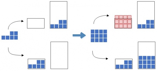
Fig. 4. Options for moving stocks into containers of different capacities.
In Figure 4, the red color represents the volume of stocks that no longer fit into the container at the second stage of placing subsequent goods.
The following requirements for the computed solutions of the problem will help correlate cubic meters of container selection costs with seconds of movement costs:
- It is necessary that the stocks from the donor cell be moved to the container cell in any case if it reduces the total number of container cells in which the goods are located.
- It is necessary to maintain a balance between the volumes of containers and the time costs of movement: for example, if in the new solution variant compared to the previous solution variant, the gain in volume is significant, while the loss in time costs is small, then the new variant should be chosen.
Let's start with the last requirement. To specify the ambiguous word 'balance', we conducted a survey of warehouse employees to find out the following. Suppose there is a container cell with a volume  , to which the movement of goods from donor cells is assigned and the total time of such movement is equal to
  Suppose there are several alternative options for placing the same amount of goods from the same donor cells into other containers, where each placement has its own assessments.
  , where
  <
< and
and  , where
  >
> .
.
The question arises: what is the minimum volume gain  acceptable, given a specified time loss.
  ? Поясним на примере. Изначально остатки полагалось размещать в контейнер объема 1000 дм3 (1 м3) и время на перемещение составило 70 секунд. Есть вариант размещения остатков в другой контейнер объема 500 дм3 и временем 130 секунд. Вопрос: готовы ли мы тратить еще дополнительные 60 секунд времени кладовщика на выполнение перемещения для того, чтобы сэкономить 500 дм3 свободного объема? По результатам опроса сотрудников склада была составлена следующая диаграмма.
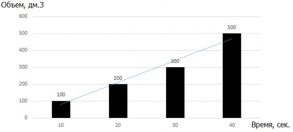
Fig. 5. Chart of the relationship between the minimum allowable volume savings and the increase in time difference for the operation.
That is, if the additional time costs amount to 40 seconds, we are only willing to incur them if the volume gain is at least 500 dm3. Despite the slight non-linearity observed in the relationship, for simplicity in further calculations, we will assume that the relationship between the quantities is linear and described by an inequality.

In the figure below, we will consider the following methods of placing goods in containers.
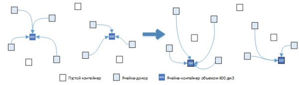
Fig. 6. Option (a): 2 containers, total volume 400 dm3, total time 150 sec.
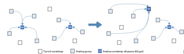
Fig. 6. Option (b): 2 containers, total volume 600 dm3, total time 190 sec.
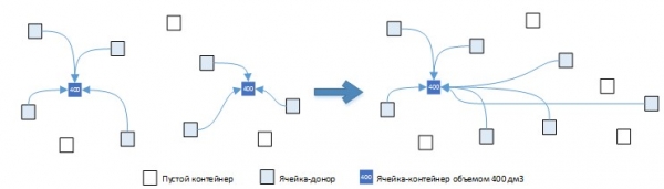
Fig. 6. Option (c): 1 container, total volume 400 dm3, total time 200 sec.
Option (a) for choosing containers is more preferred than the initial option, as the inequality is satisfied: (800-400)/10 >= 150-120, which leads to 40 >= 30. Option (b) is less preferred than the initial option since the inequality is not satisfied: (800-600)/10 >= 190-150, which leads to 20 >= 40. But option (c) does not fit into such logic! Let's examine this option in more detail. On one hand, the inequality (800-400)/10 >= 200-120 holds, which means the inequality 40 >= 80 is not satisfied, indicating that the volume gain does not justify such a significant time loss.
On the other hand, in such option (c), we are not only reducing the total occupied volume but also decreasing the number of occupied cells, which is the first of two important requirements for computed solutions to the problems listed above. Clearly, for this requirement to start being fulfilled, we need to add a certain positive constant to the left side of the inequality.  , and this constant should only be added when the number of containers decreases. Recall that
  — is a variable equal to 1 when the container
  is chosen, and 0 when the container.
  not selected. Let's designate,
  – a multitude of containers in the original solution and
  – a multitude of containers in the new solution. In general form, the new inequality will look like this:

Transforming the inequality above, we obtain

Based on this, we have a formula for calculating the total cost  of a certain variant of the task solution:

But now the question arises: what value should such a constant have  ? Очевидно, что ее значение должно быть достаточно большим, для того, чтобы всегда выполнялось первое требование к решениям задачи. Можно конечно взять значение константы равное 103 или 106, но хотелось бы избежать таких «magic numbers». Если будем рассматривать специфику выполнения складских операций, мы можем вычислить несколько вполне обоснованных числовых оценок величины такой константы.
Let  – the maximum distance between warehouse cells in one zone ABC, equal to 100 m in our case. Let
  – the maximum volume of a cell-container in the warehouse, equal to 1000 dm3 in our case.
The first method of calculating the magnitude  . Let's consider a situation where there are 2 containers on the first tier, which already physically contain goods, meaning they are themselves donor cells, and the costs of moving goods to the same cells are naturally zero. It is necessary to find such a value of the constant
  , at which it would always be profitable to move leftovers from container 1 to container 2. Substituting values
  and
and  into the inequality given above, we obtain:

from which it follows

Substituting the average execution time of elementary operations into the formula above, we get

The second method of calculating the magnitude  . Let's consider a situation where there are
  donor cells from which it is planned to move goods into container 1. Let's denote
  – the distance from the donor cell
  to container 1. There is also container 2, which already contains goods, and its volume allows accommodating leftovers from all
  cells. For simplicity, let’s assume that the volume of goods being moved from donor cells to containers is the same and equals
  . It is required to determine such a value of the constant
  , at which placing all leftovers from
  cells in container 2 would always be more profitable than placing them in different containers:

Transforming the inequality, we get

To 'enhance' the value of the magnitude  , let’s assume that
  = 0. The average number of cells usually involved in the procedure of compressing leftovers in the warehouse equals 10. Substituting the known values of the magnitudes, we have the following value for the constant

Taking the largest value computed for each variant, this will be the value of the magnitude  for the given parameters of the warehouse. Now, to complete, let’s write the formula for calculating the total costs
  for a certain permissible solution
  :
:

Now, after all the titanic efforts to transform the input data, we can say that all input data has been transformed into the required format and is ready for use in the optimization algorithm.
Conclusion
As practice shows, the labor intensity and importance of the data preparation and transformation stage for the algorithm is often underestimated. In this article, we specifically paid a lot of attention to this stage to show that only well-prepared input data can make the solutions computed by the algorithm truly valuable for the client. Yes, there were many formula outputs, but we warned you about this earlier 🙂
In the next article, we will finally get to the purpose of the previous two publications – the discrete optimization algorithm.
The article was prepared by
Roman Shangin, a programmer in the project department,
First Bit Company, Chelyabinsk
Source: habr.com
