

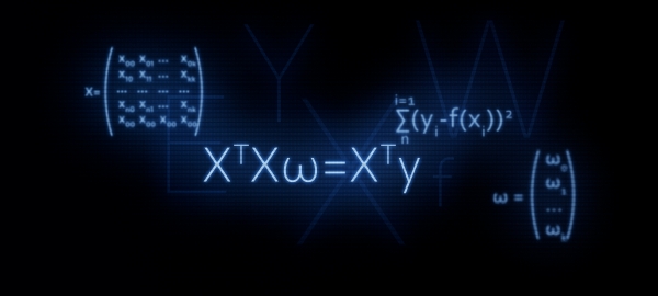
The purpose of this article is to support novice data scientists. In simple terms, we analyzed three methods for solving the linear regression equation: analytical solution, gradient descent, and stochastic gradient descent. For the analytical solution, we used the formula  . In this article, as the title suggests, we will justify the use of this formula or, in other words, derive it ourselves.
Why it makes sense to pay special attention to the formula  ?
?
It is with the matrix equation that introductions to linear regression typically begin. However, detailed derivations of how the formula was derived are rarely encountered.
For example, in Yandex's machine learning courses, when students are introduced to regularization, they are advised to use functions from the library sklearn, yet there is no mention of the matrix representation of the algorithm. This is the moment when some students may feel inclined to delve deeper into the issue—writing code without using the built-in functions. To achieve this, one must first represent the equation with the regularizer in matrix form. This article will indeed help those who wish to master such skills. Let's get started.
Initial Conditions
Target Indicators
We have a series of values for the target indicator. For example, the target indicator could be the price of an asset: oil, gold, wheat, or the dollar, etc. By a series of values of the target indicator, we mean the number of observations. Such observations could be, for instance, the monthly oil prices over a year, which means we will have 12 values for the target indicator. Let's start by introducing notations. We will denote each value of the target indicator as  . Overall, we have
  observations, and thus we can represent our observations as
  .
.
Regressors
Let's assume that there are factors that, to a certain extent, explain the values of the target variable. For example, the exchange rate of the dollar/ruble is strongly influenced by the price of oil, the Federal Reserve rate, and others. Such factors are called regressors. In this case, each value of the target variable should correspond to a value of the regressor, meaning that if we have 12 target values for each month in 2018, we should also have 12 regressor values for the same period. We denote the values of each regressor as  . Suppose that in our case there are
  regressors (i.e.,
  factors that influence the values of the target variable). This means our regressors can be represented as follows: for the 1st regressor (for example, the price of oil):
  , for the 2nd regressor (for example, the Federal Reserve rate):
  , for the "
 -th" regressor:
The dependence of the target variables on the regressors
Let’s assume that the dependence of the target variable  on the regressors "
 -th" observation can be expressed through a linear regression equation of the form:

, where  — «
— « -th" value of the regressor from 1 to
  ,
,
 - the number of regressors from 1 to
 - the coefficients that represent the magnitude by which the calculated target variable will change on average with a change in the regressor.
In other words, we determine a "unique" coefficient for each regressor (except for  ), then we multiply the coefficients by the values of the regressors for the "
  -th" observation, resulting in an approximation of the "
 -th" target variable.
 Therefore, we need to find coefficients
, for which the values of our approximating function  will be positioned as close as possible to the values of the target variables.
  Assessment of the quality of the approximating function
We will define the quality of the approximating function using the method of least squares. The quality assessment function will take the following form:
We need to find values for the coefficients $w$, for which the value

will be minimal.  We convert the equation into matrix form
Vector representation
To start, to make life easier, we should pay attention to the linear regression equation and notice that the first coefficient
To start with, to make your life easier, you should pay attention to the linear regression equation and notice that the first coefficient  is not multiplied by any regressors. Consequently, when we convert the data into matrix form, this circumstance will seriously complicate the calculations. In this regard, it is proposed to introduce another regressor for the first coefficient
  and set it to one. More precisely, each "
 -th" value of this regressor will be set to one — since multiplying by one will not change our computational results, and from the perspective of matrix multiplication rules, it will significantly reduce our struggles.
Now, for a while, to simplify the material, let’s assume we have only one " -th" observation. Then, let's represent the regressor values of the "
 -th" observation as a vector
  . The vector
  has a dimension of
  , which means
  rows and 1 column:

The sought coefficients can be represented as a vector  , which has a dimension of
  :
:

The linear regression equation for the " -th" observation will take the form:

The function for evaluating the quality of the linear model will take the form:

Note that according to the rules of matrix multiplication, we needed to transpose the vector  .
.
Matrix representation
As a result of multiplying the vectors, we will get a number:  , which was to be expected. This number is the approximation of the "
 -th" target indicator. However, we need an approximation of not just one target indicator but all of them. To achieve this, let's write all the "
 -th" regressors in matrix format
  . The resulting matrix has a dimension of
  :
:

Now the linear regression equation will take the form:

Let's denote the values of the target indicators (all  ) as a vector
  with a dimension of
  :
:

Now we can write the equation evaluating the quality of the linear model in matrix format:

In fact, from this formula, we subsequently obtain the well-known formula 
How is this done? Parentheses are expanded, differentiation is performed, the resulting expressions are transformed, etc., and this is exactly what we will now engage in.
Matrix transformations
Let’s expand the parentheses


Prepare the equation for differentiation
For this, we will perform some transformations. In the subsequent calculations, it will be more convenient if the vector  is presented at the beginning of each product in the equation.
Transformation 1

How did this happen? To answer this question, it's enough to look at the sizes of the multiplied matrices and see that we obtain a number or otherwise  .
.
Let's write down the dimensions of the matrix expressions.


Transformation 2

Let's outline similarly to transformation 1


On the output, we obtain an equation that we need to differentiate:

Let's differentiate the quality assessment function of the model
We will differentiate with respect to the vector  :
:


There should be no questions as to why  but we will consider the operations for determining the derivatives in the two other expressions in more detail.
Differentiation 1
Let's break down the differentiation: 
To determine the derivative of a matrix or vector, we need to look at their contents. Let's take a look:


We will denote the product of matrices  as a matrix
  . The matrix
  is square and moreover, it is symmetric. These properties will be useful later, let's remember them. The matrix
  has a dimension of
  :
:

Now our task is to correctly multiply the vectors by the matrix and avoid getting 'two times two equals five,' so let's focus and be extremely careful.


However, we ended up with an intricate expression! In fact, we have obtained a number—a scalar. And now, we are truly transitioning to differentiation. We need to find the derivative of the obtained expression with respect to each coefficient  and we will get an output vector of size
  . Just in case, I will describe the procedures step by step:
1) differentiate with respect to  , we will obtain:
2) differentiate with respect to  , we will obtain:
3) differentiate with respect to  , we will obtain:
On output—the promised vector of size  :
:

If we look closely at the vector, we can notice that the left and corresponding right elements of the vector can be grouped in such a way that ultimately, from the presented vector, we can extract a vector  of size
  . For example,
  (the left element of the top row of the vector)
  (the right element of the top row of the vector) can be represented as
  , and
, and  — as
— as  and so on for each row. Let's group them:

We will factor out the vector  and we will obtain:

Now, let's take a closer look at the resulting matrix. The matrix represents the sum of two matrices  :
:

Let's remember that some time ago, we pointed out one important property of the matrix  — it is symmetric. Based on this property, we can confidently state that the expression
  is equal to
  . This is easy to verify by expanding the matrix multiplication element-wise.
  We won't do this here, those interested can conduct the check themselves.
Let's return to our expression. After our transformations, it turned out just as we wanted to see it:

So, we have managed the first differentiation. Now, let's move on to the second expression.
Differentiation 2

Let's take the beaten path. It will be much shorter than the previous one, so don't stray far from the screen.
Let's break down the vectors and the matrix element by element:


For now, let's remove the two from the calculations — it doesn't play a significant role, and we'll put it back later. We'll multiply the vectors by the matrix. First, we will multiply the matrix  by the vector
  , here we have no restrictions. We'll get a vector of size
  :
:

Next, we will perform the following operation — multiply the vector  by the resulting vector. We will end up with a number:

This is what we will differentiate. We will get a vector of dimension  :
:

Does this remind you of something? That's right! This is the product of the matrix  by the vector
  .
.
Thus, the second differentiation is successfully completed.
In conclusion
Now we know how the equality was derived  .
.
Finally, let's outline a quick way to transform the basic formulas.
We will assess the model's quality according to the least squares method:


Let's differentiate the obtained expression:


Literature
Internet sources:
1)
2)
3)
4)
Textbooks, problem sets:
1) Lecture notes on higher mathematics: complete course / D.T. Pismennyi – 4th ed. – Moscow: Iris-Press, 2006
2) Applied regression analysis / N. Draper, G. Smith – 2nd ed. – Moscow: Finance and Statistics, 1986 (translated from English)
3) Problems on solving matrix equations:
Source: habr.com
