

In this article, we will discuss functional dependencies in databases — what they are, where they are applied, and what algorithms exist for their discovery.
We will consider functional dependencies in the context of relational databases. To put it simply, in such databases, information is stored in the form of tables. Next, we will use approximate terms that are not interchangeable in strict relational theory: we will call the table a relation, the columns attributes (their entirety is the relation's schema), and the set of values in a row over a subset of attributes a tuple.
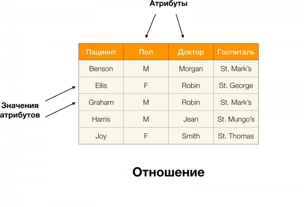
For example, in the table above, (Benson, M, M organ) is a tuple across the attributes (Patient, Gender, Doctor).
More formally, this is written as follows:  [Patient, Gender, Doctor] = (Benson, M, M organ).
Now we can introduce the concept of functional dependency (FD):
Definition 1. A relation R satisfies FD X → Y (where X, Y ⊆ R) if and only if for any tuples  ,
,  ∈ R, it holds: if
  [X] =
[X] =  [X], then
  [Y] =
[Y] =  [Y]. In this case, it is said that X (the determinant, or defining set of attributes) functionally determines Y (the dependent set).
In other words, the presence of FD X → Y means that if we have two tuples in R that agree on the attributes X, then they will also agree on the attributes Y.
Now in order. Let’s consider the attributes Patient and Gender for which we want to find out whether there are dependencies among them. For such a set of attributes, the following dependencies may exist:
- Patient → Gender
- Gender → Patient
According to the definition above, for the first dependency to hold, each unique value of the column Patient must correspond to only one value of the column Gender. And for the sample table, this is indeed the case. However, this does not work in reverse, meaning the second dependency does not hold, and the attribute Gender is not a determinant for Patient.Similarly, if we take the dependency Doctor → Patient, we can notice that it is violated since the value of Robin for this attribute has several different values — Ellis and Graham..
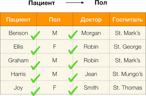
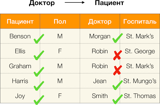
Thus, functional dependencies allow us to identify existing relationships between sets of attributes in a table. From now on, we will focus on the most interesting relationships, namely those X → Y, which are:
- non-trivial, meaning that the right side of the dependency is not a subset of the left (Y ̸⊆ X);
- minimal, meaning there is no such dependency Z → Y, that Z ⊂ X.
The dependencies considered thus far have been strict, meaning they do not allow for any violations in the table, but besides them, there are those that permit some inconsistency between the values of tuples. Such dependencies are placed in a separate class, called approximate, and are allowed to be violated for a certain number of tuples. This number is regulated by the maximum error indicator emax. For example, an error rate  = 0.01 may indicate that the dependency can be violated in 1% of the existing tuples in the considered set of attributes. This means that for 1000 records, a maximum of 10 tuples may violate the functional dependency. However, we will consider a slightly different metric based on pairwise distinct values of the compared tuples. For the dependency X → Y on the relation r it is calculated as follows:

Let's calculate the error for Doctor → Patient the example above. We have two tuples whose values differ in the attribute Patient, but match on Doctor:  [Doctor, Patient] = (Robin, Ellis) and
  [Doctor, Patient] = (Robin, Graham). Following the definition of error, we must consider all conflicting pairs, which means there will be two: (
 ,
,  ) and its inversion (
 ,
,  ). Substituting into the formula, we get:

And now we will attempt to answer the question: 'What is it all for?'. In fact, functional dependencies can vary. The first type consists of dependencies defined by the administrator during the database design phase. They are usually few in number, are strict, and their main application is data normalization and relation schema design.
The second type consists of dependencies representing "hidden" data and previously unknown relationships between attributes. This means that such dependencies were not considered at the time of design and they are discovered only when analyzing an existing dataset, enabling conclusions about the stored information to be drawn based on the multitude of identified functional dependencies. This is precisely the type of dependencies we work with. A whole field of data mining deals with these, employing various search techniques and algorithms built upon them. Let's explore how identified functional dependencies (exact or approximate) can be useful in any data.

Today, one of the main areas of application for dependencies is data cleansing. This involves developing processes to identify "dirty data" followed by their correction. Typical examples of "dirty data" include duplicates, data entry errors or typos, missing values, outdated information, extra spaces, and so on.
Example of a data error:
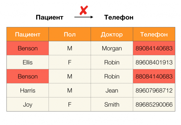
Example of duplicates in data:
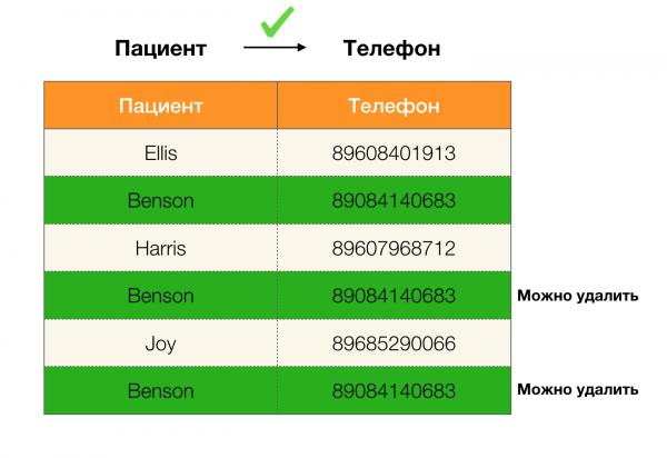
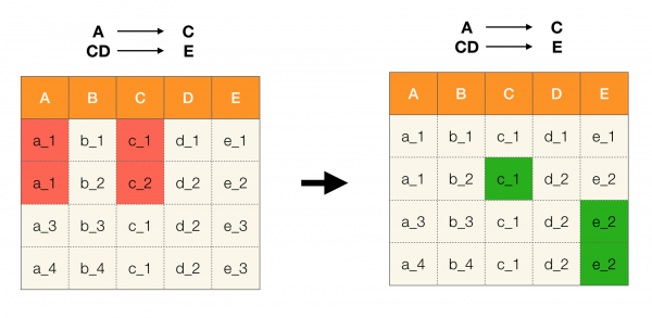
For instance, we have a table and a set of functional dependencies that must be satisfied. Data cleansing in this case means altering the data so that the functional dependencies become valid. The number of modifications should be minimal (there are specific algorithms for this process, which we will not focus on in this article). Below is an example of such data transformation. On the left is the original relation, where the required functional dependencies are obviously not met (an example of a violation of one of the dependencies is highlighted in red). On the right is the updated relation, where the green cells indicate the modified values. After conducting this procedure, the necessary dependencies began to hold.
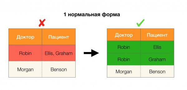
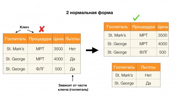
Another popular application area is database design. Here, it is worth mentioning normal forms and normalization. Normalization is the process of bringing a relation into compliance with a certain set of requirements, each of which is defined by a normal form in its own way. We will not elaborate on the requirements of different normal forms (this is addressed in any introductory database textbook), but will note that each one uses the concept of functional dependencies in its own way. After all, functional dependencies are essentially integrity constraints considered during database design (in this context, functional dependencies are sometimes referred to as superkeys).
Let's consider their application for the four normal forms in the image below. Remember that the Boyce-Codd normal form is stricter than the third form but less strict than the fourth. We will not cover the latter yet, as it requires an understanding of multi-valued dependencies, which are not of interest to us in this article.
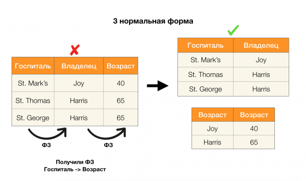
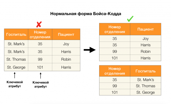
Another area where dependencies have found their application is in reducing the dimensionality of feature spaces in tasks such as building a naive Bayes classifier, highlighting significant features, and reparameterizing regression models. In original articles, this task is referred to as determining feature redundancy and relevancy, and it is actively addressed using database concepts. With the emergence of such works, we can say that there is currently a demand for solutions that allow the integration of databases, analytics, and the implementation of the aforementioned optimization problems into a single tool.
There are many algorithms for searching functional dependencies in datasets (both modern and not so modern). These algorithms can be divided into three groups:
- Algorithms that use lattice traversal
- Algorithms based on finding consistent values
- Algorithms based on pairwise comparisons
A brief description of each type of algorithm is presented in the table below:
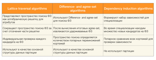
Learn more about this classification [4]. Below are examples of algorithms for each type:
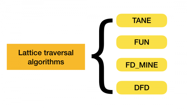
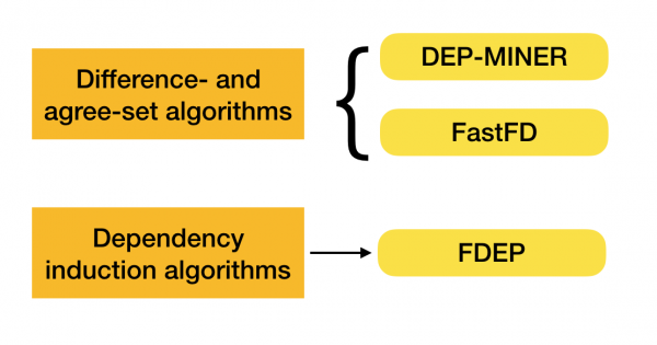
Currently, new algorithms are emerging that combine several approaches to finding functional dependencies. Examples of such algorithms include Pyro [2] and HyFD [3]. Their workings will be discussed in the following articles in this series. In this article, we will only cover the basic concepts and lemmas necessary for understanding the techniques for identifying dependencies.
Let's start with the basics — difference-set and agree-set, used in the second type of algorithms. The difference-set is a set of tuples that do not match in values, while the agree-set consists of tuples that match in values. It should be noted that in this case we are only considering the left side of the dependency.
Another important concept mentioned above is the algebraic lattice. Since many modern algorithms operate with this concept, we need to understand what it entails.
To introduce the concept of a lattice, we need the definition of a partially ordered set (or poset).
Definition 2. A set S is said to be partially ordered by a binary relation ⩽ if for any a, b, c ∈ S the following properties hold:
- Reflexivity, meaning a ⩽ a
- Antisymmetry, meaning if a ⩽ b and b ⩽ a, then a = b
- Transitivity, meaning for a ⩽ b and b ⩽ c it follows that a ⩽ c
Such a relation is called a (non-strict) partial order, and the set itself is called a partially ordered set. Formal notation: ⟨S, ⩽⟩.
As a simple example of a partially ordered set, consider the set of all natural numbers N with the usual order relation ⩽. It is not difficult to verify that all necessary axioms are satisfied.
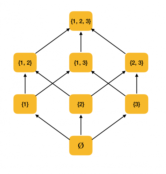
A more substantial example. Consider the set of all subsets {1, 2, 3}, ordered by the inclusion relation ⊆. Indeed, this relation satisfies all the conditions of a partial order, thus ⟨P ({1, 2, 3}), ⊆⟩ is a partially ordered set. The structure of this set is illustrated below: if one element can reach another by following the arrows, then they are in an order relation.
We will need two more simple definitions from the field of mathematics — supremum and infimum.
Definition 3. Let ⟨S, ⩽⟩ be a partially ordered set, A ⊆ S. An upper bound of A is an element u ∈ S such that ∀x ∈ S: x ⩽ u. Let U be the set of all upper bounds of S. If there exists a least element in U, it is called the supremum and is denoted as sup A.
Similarly, the concept of exact lower bound is introduced.
Definition 4. Let ⟨S, ⩽⟩ be a partially ordered set, A ⊆ S. A lower bound of A is an element l ∈ S such that ∀x ∈ S: l ⩽ x. Let L be the set of all lower bounds of S. If there exists a greatest element in L, it is called the infimum and is denoted as inf A.
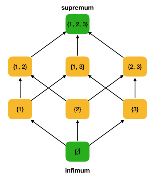
As an example, let us consider the partially ordered set ⟨P ({1, 2, 3}), ⊆⟩ and find the supremum and infimum in it:
Now we can formulate the definition of an algebraic lattice.
Definition 5. Let ⟨P, ⩽⟩ be a partially ordered set such that every two-element subset has exact upper and lower bounds. Then P is called an algebraic lattice. Here, sup{x, y} is written as x ∨ y, and inf {x, y} as x ∧ y.
Let's verify that our working example ⟨P ({1, 2, 3}), ⊆⟩ is a lattice. Indeed, for any a, b ∈ P ({1, 2, 3}), a ∨ b = a ∪ b, and a ∧ b = a ∩ b. For example, consider the sets {1, 2} and {1, 3} and find their infimum and supremum. If we intersect them, we get the set {1}, which will be the infimum. The supremum will be their union — {1, 2, 3}.
In algorithms for discovering functional dependencies, the search space is often represented in the form of a lattice, where sets of a single element (think of the first level of the search lattice, where the left part of dependencies consists of a single attribute) represent each attribute of the original relation.
Initially, dependencies of the form ∅ → are considered. A single attribute. This step helps to identify which attributes are primary keys (for such attributes, there are no determinants, hence the left part is empty). Further, such algorithms move upwards through the lattice. It should be noted that the lattice does not need to be traversed entirely; that is, if a desired maximum size of the left part is provided as input, the algorithm will not proceed beyond the level with that size.
The illustration below shows how an algebraic lattice can be used in a functional dependency search task. Here, each edge (X, XY) represents a dependency X → Y. For example, we passed the first level and know that the dependency A → B (we will represent this with a green link between the nodes A and B). This means that when we move up the lattice, we do not need to check the dependency A, C → B, because it will already not be minimal. Similarly, we wouldn’t check it if the dependency C → B.
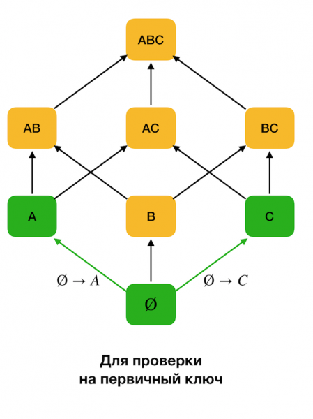
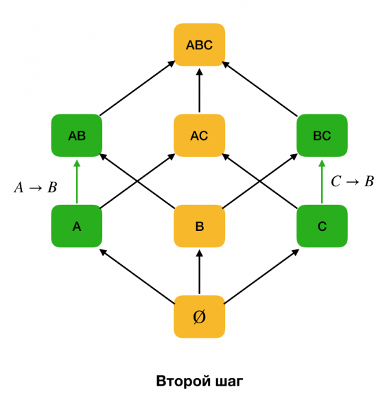
were maintained. Moreover, generally, all modern algorithms for functional dependency search use a data structure known as partition (in the source — stripped partition [1]). The formal definition of a partition is as follows:
Definition 6. Let X ⊆ R be a set of attributes for relation r. A cluster is a set of tuple indices from r that have the same value for X, that is, c(t) = {i|ti[X] = t[X]}. A partition is a set of clusters, excluding unit-length clusters:

In simpler terms, a partition for attribute X is a set of lists, where each list contains row numbers with the same values for X. In modern literature, the structure representing partitions is called position list index (PLI). Unit-length clusters are excluded for the sake of compressing PLI, because these are clusters containing only the record number with a unique value, which will always be easy to determine.
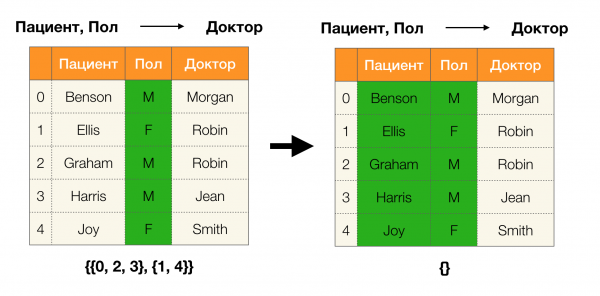
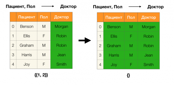
Let’s consider an example. Let’s return to the same table of patients and build partitions for the columns Patient and Gender (a new column has appeared on the left, indicating the row numbers of the table):
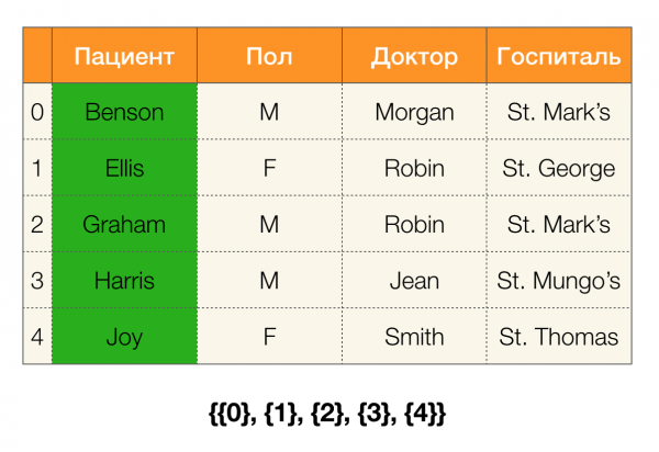
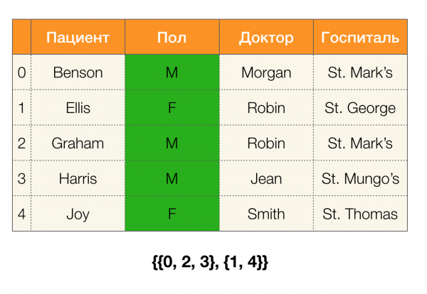
According to the definition, however, the partition for the column Patient will actually be empty, as single clusters are excluded from the partition.
Partitions can be generated across multiple attributes. There are two ways to do this: by traversing the table to build a partition across all necessary attributes at once, or by constructing it via the intersection of partitions across a subset of attributes. Dependency search algorithms use the second option.
In simpler terms, to obtain a partition by the columns ABC, one can take the partitions for AC and B (or any other set of non-overlapping subsets) and intersect them. The intersection operation of two partitions highlights the longest clusters common to both partitions.
Let's consider an example:
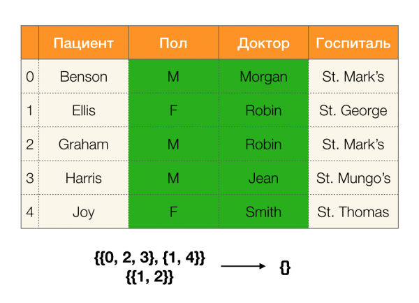
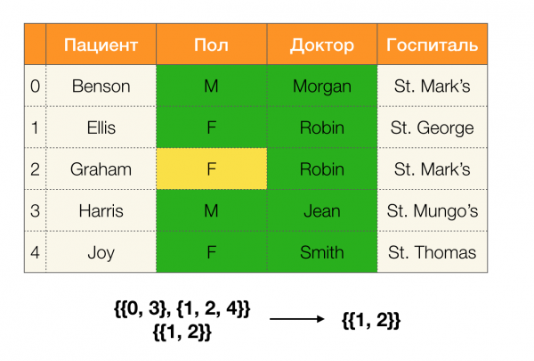
In the first case, we obtained an empty partition. If you look closely at the table, there are indeed no identical values for the two attributes. If we slightly modify the table (the case on the right), we will get a non-empty intersection. In this case, rows 1 and 2 do indeed have the same values for the attributes. Gender and Doctor.
Next, we will need a concept called partition size. Formally:

In simpler terms, the size of the partition represents the number of clusters included in the partition (remember, single clusters do not count towards the partition!):
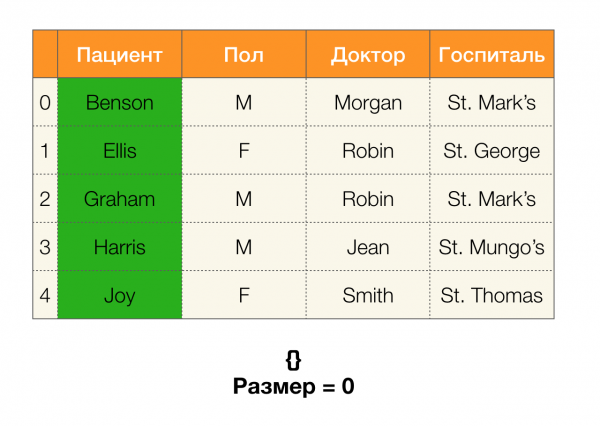
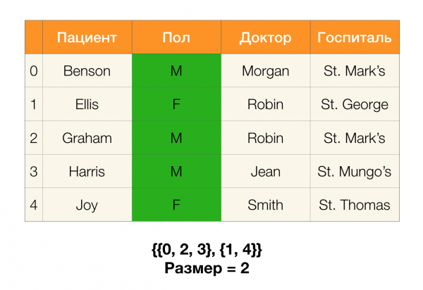
Now we can define one of the key lemmas that allows us to determine whether a dependency is maintained for the given partitions:
Lemma 1. The dependency A, B → C is maintained if and only if

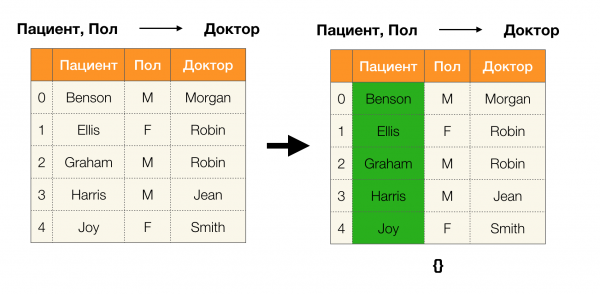
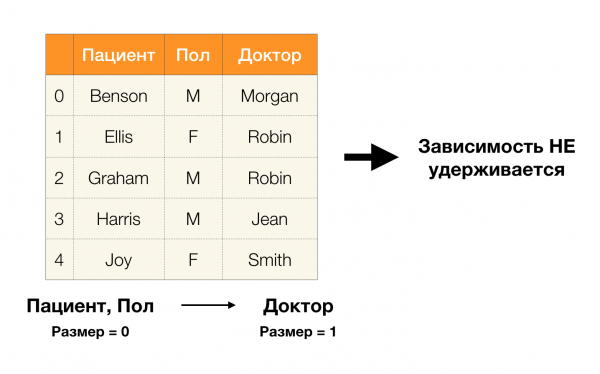
According to the lemma, to determine whether a dependency is maintained, four steps must be performed:
- Calculate the partition for the left side of the dependency
- Calculate the partition for the right side of the dependency
- Calculate the product of the first and second steps
- Compare the sizes of the partitions obtained in the first and third steps
Below is an example of checking whether the dependency is maintained according to this lemma:
In this article, we discussed concepts such as functional dependency, approximate functional dependency, where they are applied, and what algorithms for finding FD exist. We also thoroughly examined basic but important concepts actively used in modern algorithms for finding FDs.
References:
- Huhtala Y. et al. TANE: An efficient algorithm for discovering functional and approximate dependencies // The computer journal. – 1999. – Vol. 42. – No. 2. – P. 100-111.
- Kruse S., Naumann F. Efficient discovery of approximate dependencies // Proceedings of the VLDB Endowment. – 2018. – Vol. 11. – No. 7. – P. 759-772.
- Papenbrock T., Naumann F. A hybrid approach to functional dependency discovery // Proceedings of the 2016 International Conference on Management of Data. – ACM, 2016. – P. 821-833.
- Papenbrock T. et al. Functional dependency discovery: An experimental evaluation of seven algorithms // Proceedings of the VLDB Endowment. – 2015. – Vol. 8. – No. 10. – P. 1082-1093.
- Kumar A. et al. To join or not to join?: Thinking twice about joins before feature selection // Proceedings of the 2016 International Conference on Management of Data. – ACM, 2016. – P. 19-34.
- Abo Khamis M. et al. In-database learning with sparse tensors // Proceedings of the 37th ACM SIGMOD-SIGACT-SIGAI Symposium on Principles of Database Systems. – ACM, 2018. – P. 325-340.
- Hellerstein J. M. et al. The MADlib analytics library: or MAD skills, the SQL // Proceedings of the VLDB Endowment. – 2012. – Vol. 5. – No. 12. – P. 1700-1711.
- Qin C., Rusu F. Speculative approximations for terascale distributed gradient descent optimization // Proceedings of the Fourth Workshop on Data analytics in the Cloud. – ACM, 2015. – P. 1.
- Meng X. et al. Mllib: Machine learning in apache spark // The Journal of Machine Learning Research. – 2016. – Vol. 17. – No. 1. – P. 1235-1241.
Authors of the article: , researcher at , and , researcher at
Source: habr.com
