


Hello, Habr!
Last autumn, a competition was held on Kaggle for classifying hand-drawn images in the Quick Draw Doodle Recognition, where a team of R enthusiasts participated, consisting of , and . We won't go into detail about the competition, as this has already been covered in a .
. While we didn't achieve a medal farm this time, we gained a lot of valuable experience, and we would like to share some of the most interesting and useful insights from Kaggle and our daily work with the community. The topics discussed include the tough life without OpenCV, JSON parsing (these examples examine integrating C++ code into R scripts or packages using Rcpp), script parameterization, and dockerization of the final solution. All the code from the message is available in a runnable format at .
Contents:
1. Effective Data Loading from CSV to MonetDB
The data in this competition is provided not as ready-made images, but as 340 CSV files (one for each class), containing JSON files with point coordinates. Connecting these points with lines yields the final image sized 256x256 pixels. Each entry also includes a label indicating whether the image was correctly recognized by the classifier used at the time of dataset collection, a two-letter country code of the drawing's author, a unique identifier, a timestamp, and a class name matching the filename. A simplified version of the original data weighs 7.4 GB in the archive and about 20 GB when unpacked; the full data occupies 240 GB after unpacking. The organizers guaranteed that both versions reproduce the same drawings, meaning the full version is redundant. In any case, storing 50 million images as graphic files or arrays was immediately deemed unfeasible, and we decided to combine all the CSV files from the archive train_simplified.zip into a database, with subsequent generation of images of the required size 'on-the-fly' for each batch.
A well-proven DBMS was chosen. RE2, specifically the implementation for R as a package . The package includes an embedded version of the database server and allows you to launch the server directly from the R session and work with it there. Creating a database and connecting to it can be done in one command:
con <- DBI::dbConnect(drv = MonetDBLite::MonetDBLite(), Sys.getenv("DBDIR"))We will need to create two tables: one for all data, and another for metadata about the uploaded files (useful if something goes wrong and the process needs to be resumed after uploading multiple files):
Creating tables
if (!DBI::dbExistsTable(con, "doodles")) {
  DBI::dbCreateTable(
    con = con,
    name = "doodles",
    fields = c(
      "countrycode" = "char(2)",
      "drawing" = "text",
      "key_id" = "bigint",
      "recognized" = "bool",
      "timestamp" = "timestamp",
      "word" = "text"
    )
  )
}

if (!DBI::dbExistsTable(con, "upload_log")) {
  DBI::dbCreateTable(
    con = con,
    name = "upload_log",
    fields = c(
      "id" = "serial",
      "file_name" = "text UNIQUE",
      "uploaded" = "bool DEFAULT false"
    )
  )
}
The fastest way to upload data into the database was to directly copy CSV files using SQL — the command COPY OFFSET 2 INTO tablename FROM path USING DELIMITERS ',', 'n', '"' NULL AS '' BEST EFFORT, where tablename — the table name and — Specifies the path in the container to which LXD will mount this device. — the path to the file. In working with the archive, it was found that the built-in implementation unzip in R works incorrectly with several files from the archive, so we used the system's unzip (using the parameter getOption("unzip")).
Function for writing to the database
#' @title Извлечение и загрузка файлов
#'
#' @description
#' Извлечение CSV-файлов из ZIP-архива и загрузка их в базу данных
#'
#' @param con Объект подключения к базе данных (класс `MonetDBEmbeddedConnection`).
#' @param tablename Название таблицы в базе данных.
#' @oaram zipfile Путь к ZIP-архиву.
#' @oaram filename Имя файла внури ZIP-архива.
#' @param preprocess Функция предобработки, которая будет применена извлечённому файлу.
#'   Должна принимать один аргумент `data` (объект `data.table`).
#'
#' @return `TRUE`.
#'
upload_file <- function(con, tablename, zipfile, filename, preprocess = NULL) {
  # Проверка аргументов
  checkmate::assert_class(con, "MonetDBEmbeddedConnection")
  checkmate::assert_string(tablename)
  checkmate::assert_string(filename)
  checkmate::assert_true(DBI::dbExistsTable(con, tablename))
  checkmate::assert_file_exists(zipfile, access = "r", extension = "zip")
  checkmate::assert_function(preprocess, args = c("data"), null.ok = TRUE)

  # Извлечение файла
  path <- file.path(tempdir(), filename)
  unzip(zipfile, files = filename, exdir = tempdir(),
        junkpaths = TRUE, unzip = getOption("unzip"))
  on.exit(unlink(file.path(path)))

  # Применяем функция предобработки
  if (!is.null(preprocess)) {
    .data <- data.table::fread(file = path)
    .data <- preprocess(data = .data)
    data.table::fwrite(x = .data, file = path, append = FALSE)
    rm(.data)
  }

  # Запрос к БД на импорт CSV
  sql <- sprintf(
    "COPY OFFSET 2 INTO %s FROM '%s' USING DELIMITERS ',','n','"' NULL AS '' BEST EFFORT",
    tablename, path
  )
  # Выполнение запроса к БД
  DBI::dbExecute(con, sql)

  # Добавление записи об успешной загрузке в служебную таблицу
  DBI::dbExecute(con, sprintf("INSERT INTO upload_log(file_name, uploaded) VALUES('%s', true)",
                              filename))

  return(invisible(TRUE))
}
If you need to transform the table before writing it to the database, simply pass a function that will transform the data as an argument. preprocess Code for sequentially loading data into the database:
Writing data to the database
The data upload time may vary depending on the speed characteristics of the storage used. In our case, reading and writing from one SSD or transferring from a flash drive (source file) to SSD (database) takes less than 10 minutes.
# Список файлов для записи
files <- unzip(zipfile, list = TRUE)$Name

# Список исключений, если часть файлов уже была загружена
to_skip <- DBI::dbGetQuery(con, "SELECT file_name FROM upload_log")[[1L]]
files <- setdiff(files, to_skip)

if (length(files) > 0L) {
  # Запускаем таймер
  tictoc::tic()
  # Прогресс бар
  pb <- txtProgressBar(min = 0L, max = length(files), style = 3)
  for (i in seq_along(files)) {
    upload_file(con = con, tablename = "doodles",
                zipfile = zipfile, filename = files[i])
    setTxtProgressBar(pb, i)
  }
  close(pb)
  # Останавливаем таймер
  tictoc::toc()
}

# 526.141 sec elapsed - копирование SSD->SSD
# 558.879 sec elapsed - копирование USB->SSD
A few more seconds are needed to create a column with an integer class label and an index column (
ORDERED INDEX) with row numbers, which will be used to sample observations when creating batches:Creating additional columns and an index
message("Generate labels") invisible(DBI::dbExecute(con, "ALTER TABLE doodles ADD label_int int")) invisible(DBI::dbExecute(con, "UPDATE doodles SET label_int = dense_rank() OVER (ORDER BY word) - 1"))message("Generate row numbers") invisible(DBI::dbExecute(con, "ALTER TABLE doodles ADD id serial")) invisible(DBI::dbExecute(con, "CREATE ORDERED INDEX doodles_id_ord_idx ON doodles(id)"))
message("Generate labels")
invisible(DBI::dbExecute(con, "ALTER TABLE doodles ADD label_int int"))
invisible(DBI::dbExecute(con, "UPDATE doodles SET label_int = dense_rank() OVER (ORDER BY word) - 1"))

message("Generate row numbers")
invisible(DBI::dbExecute(con, "ALTER TABLE doodles ADD id serial"))
invisible(DBI::dbExecute(con, "CREATE ORDERED INDEX doodles_id_ord_idx ON doodles(id)"))
To solve the task of forming a batch 'on the fly', we needed to achieve maximum speed in extracting random rows from the table. doodlesTo do this, we employed three tricks. The first involved reducing the dimensionality of the type used to store the observation ID. In the original dataset, the type required for storing IDs is bigint, but the number of observations allows us to fit their identifiers, which are equal to their ordinal numbers, into the type int. This makes the search significantly faster. The second trick was the use of ) with row numbers, which will be used to sample observations when creating batches: — we arrived at this solution empirically, testing all available . The third involved the use of parameterized queries. The essence of the method consists of executing the command PREPARE once and subsequently using the prepared expression when creating a heap of uniform requests, but in practice, the gain compared to a simple SELECT was around statistical error.
The data loading process consumes no more than 450 MB of RAM. This means the described approach allows handling datasets weighing in tens of gigabytes on virtually any budget hardware, including some single-board computers, which is quite impressive.
We still need to measure the speed of extracting (random) data and evaluate the scalability when sampling batches of different sizes:
Database benchmark
library(ggplot2)

set.seed(0)
# Connecting to the database
con <- DBI::dbConnect(MonetDBLite::MonetDBLite(), Sys.getenv("DBDIR"))

# Function to prepare a server-side query
prep_sql <- function(batch_size) {
  sql <- sprintf("PREPARE SELECT id FROM doodles WHERE id IN (%s)",
                 paste(rep("?", batch_size), collapse = ","))
  res <- DBI::dbSendQuery(con, sql)
  return(res)
}

# Function to fetch data
fetch_data <- function(rs, batch_size) {
  ids <- sample(seq_len(n), batch_size)
  res <- DBI::dbFetch(DBI::dbBind(rs, as.list(ids)))
  return(res)
}

# Conducting the benchmark
res_bench <- bench::press(
  batch_size = 2^(4:10),
  {
    rs <- prep_sql(batch_size)
    bench::mark(
      fetch_data(rs, batch_size),
      min_iterations = 50L
    )
  }
)
# Benchmark parameters
cols <- c("batch_size", "min", "median", "max", "itr/sec", "total_time", "n_itr")
res_bench[, cols]

#   batch_size      min   median      max `itr/sec` total_time n_itr
#
# 1         16   23.6ms  54.02ms  93.43ms     18.8        2.6s    49
# 2         32     38ms  84.83ms 151.55ms     11.4       4.29s    49
# 3         64   63.3ms 175.54ms 248.94ms     5.85       8.54s    50
# 4        128   83.2ms 341.52ms 496.24ms     3.00      16.69s    50
# 5        256  232.8ms 653.21ms 847.44ms     1.58      31.66s    50
# 6        512  784.6ms    1.41s    1.98s     0.740       1.1m    49
# 7       1024  681.7ms    2.72s    4.06s     0.377      2.16m    49

ggplot(res_bench, aes(x = factor(batch_size), y = median, group = 1)) +
  geom_point() +
  geom_line() +
  ylab("median time, s") +
  theme_minimal()

DBI::dbDisconnect(con, shutdown = TRUE) 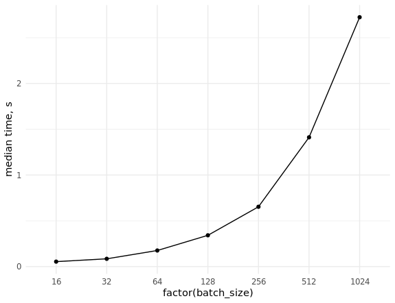
2. Preparing Batches
The entire batch preparation process consists of the following stages:
- Parsing several JSON files containing vectors of strings with coordinates of points.
- Drawing colored lines according to the point coordinates on an image of the required size (e.g., 256×256 or 128×128).
- Transforming the obtained images into a tensor.
In the context of the competition among kernels on Python, the task was primarily solved using OpenCV. One of the simplest and most straightforward equivalents in R would look as follows:
Implementing JSON to tensor transformation in R
r_process_json_str <- function(json, line.width = 3,
                               color = TRUE, scale = 1) {
  # Parsing JSON
  coords <- jsonlite::fromJSON(json, simplifyMatrix = FALSE)
  tmp <- tempfile()
  # Delete temporary file upon function completion
  on.exit(unlink(tmp))
  png(filename = tmp, width = 256 * scale, height = 256 * scale, pointsize = 1)
  # Empty plot
  plot.new()
  # Plot window size
  plot.window(xlim = c(256 * scale, 0), ylim = c(256 * scale, 0))
  # Line colors
  cols <- if (color) rainbow(length(coords)) else "#000000"
  for (i in seq_along(coords)) {
    lines(x = coords[[i]][[1]] * scale, y = coords[[i]][[2]] * scale,
          col = cols[i], lwd = line.width)
  }
  dev.off()
  # Convert image to 3D array
  res <- png::readPNG(tmp)
  return(res)
}

r_process_json_vector <- function(x, ...) {
  res <- lapply(x, r_process_json_str, ...)
  # Combine 3D image arrays into a 4D tensor
  res <- do.call(abind::abind, c(res, along = 0))
  return(res)
}
The drawing is performed using standard R tools, saving it to a temporary PNG stored in RAM (in Linux, temporary directories for R are located in a directory /tmp, mounted in RAM). Then, this file is read as a three-dimensional array with numbers ranging from 0 to 1. This is important since a more commonly used BMP would be read as a raw array with hex color codes.
Let's test the result:
zip_file <- file.path("data", "train_simplified.zip")
csv_file <- "cat.csv"
unzip(zip_file, files = csv_file, exdir = tempdir(),
      junkpaths = TRUE, unzip = getOption("unzip"))
tmp_data <- data.table::fread(file.path(tempdir(), csv_file), sep = ",",
                              select = "drawing", nrows = 10000)
arr <- r_process_json_str(tmp_data[4, drawing])
dim(arr)
# [1] 256 256   3
plot(magick::image_read(arr)) 
The batch itself will be formed as follows:
res <- r_process_json_vector(tmp_data[1:4, drawing], scale = 0.5)
str(res)
 # num [1:4, 1:128, 1:128, 1:3] 1 1 1 1 1 1 1 1 1 1 ...
 # - attr(*, "dimnames")=List of 4
 #  ..$ : NULL
 #  ..$ : NULL
 #  ..$ : NULL
 #  ..$ : NULL
This implementation seemed suboptimal to us, as forming large batches takes an unreasonably long time, and we decided to draw on the experience of our colleagues by using a powerful library OpenCV. At that time, there was no ready-made package for R (and there still isn't), so a minimal implementation of the required functionality was written in C++ with integration into R code via Rcpp.
The following packages and libraries were used to solve the task:
OpenCV for working with images and drawing lines. We used pre-installed system libraries and header files, as well as dynamic linking.
xtensor for working with multidimensional arrays and tensors. We used the header files included in the eponymous R package. The library allows handling multidimensional arrays in both row major and column major order.
ndjson for parsing JSON. This library is used in xtensor automatically if it is present in the project.
RcppThread for organizing multithreaded processing of vectors from JSONs. We used the header files provided by this package. Compared to the more popular RcppParallel package among other features has a built-in mechanism for interrupting the loop.
It should be noted that xtensor turned out to be a real find: in addition to having extensive functionality and high performance, its developers were quite responsive and promptly and thoroughly answered any questions that arose. With their help, we managed to implement transformations of OpenCV matrices into xtensor tensors, as well as a way to combine 3-dimensional image tensors into a 4-dimensional tensor of the correct size (the actual batch).
Materials for studying Rcpp, xtensor, and RcppThread
To compile files that use system files and dynamic linking with libraries installed on the system, we utilized the plugin mechanism implemented in the package Rcpp. For automatically finding paths and flags, we used the popular Linux utility pkg-config.
Implementation of the Rcpp plugin to use the OpenCV library
Rcpp::registerPlugin("opencv", function() {
  # Possible package names
  pkg_config_name <- c("opencv", "opencv4")
  # Binary file of the pkg-config utility
  pkg_config_bin <- Sys.which("pkg-config")
  # Check for utility presence in the system
  checkmate::assert_file_exists(pkg_config_bin, access = "x")
  # Check for the presence of OpenCV settings file for pkg-config
  check <- sapply(pkg_config_name,
                  function(pkg) system(paste(pkg_config_bin, pkg)))
  if (all(check != 0)) {
    stop("OpenCV config for the pkg-config not found", call. = FALSE)
  }

  pkg_config_name <- pkg_config_name[check == 0]
  list(env = list(
    PKG_CXXFLAGS = system(paste(pkg_config_bin, "--cflags", pkg_config_name),
                          intern = TRUE),
    PKG_LIBS = system(paste(pkg_config_bin, "--libs", pkg_config_name),
                      intern = TRUE)
  ))
})
As a result of the plugin's operation during compilation, the following values will be substituted:
Rcpp:::.plugins$opencv()$env

# $PKG_CXXFLAGS
# [1] "-I/usr/include/opencv"
#
# $PKG_LIBS
# [1] "-lopencv_shape -lopencv_stitching -lopencv_superres -lopencv_videostab -lopencv_aruco -lopencv_bgsegm -lopencv_bioinspired -lopencv_ccalib -lopencv_datasets -lopencv_dpm -lopencv_face -lopencv_freetype -lopencv_fuzzy -lopencv_hdf -lopencv_line_descriptor -lopencv_optflow -lopencv_video -lopencv_plot -lopencv_reg -lopencv_saliency -lopencv_stereo -lopencv_structured_light -lopencv_phase_unwrapping -lopencv_rgbd -lopencv_viz -lopencv_surface_matching -lopencv_text -lopencv_ximgproc -lopencv_calib3d -lopencv_features2d -lopencv_flann -lopencv_xobjdetect -lopencv_objdetect -lopencv_ml -lopencv_xphoto -lopencv_highgui -lopencv_videoio -lopencv_imgcodecs -lopencv_photo -lopencv_imgproc -lopencv_core"
The code for implementing JSON parsing and forming a batch for transfer to the model is provided in the spoiler. First, we add the local project directory to search for header files (needed for ndjson):
Sys.setenv("PKG_CXXFLAGS" = paste0("-I", normalizePath(file.path("src"))))Implementation of converting JSON to a tensor in C++
// [[Rcpp::plugins(cpp14)]]
// [[Rcpp::plugins(opencv)]]
// [[Rcpp::depends(xtensor)]]
// [[Rcpp::depends(RcppThread)]]

#include <xtensor/xjson.hpp>
#include <xtensor/xadapt.hpp>
#include <xtensor/xview.hpp>
#include <xtensor-r/rtensor.hpp>
#include <opencv2/core/core.hpp>
#include <opencv2/highgui/highgui.hpp>
#include <opencv2/imgproc/imgproc.hpp>
#include <Rcpp.h>
#include <RcppThread.h>

// Синонимы для типов
using RcppThread::parallelFor;
using json = nlohmann::json;
using points = xt::xtensor<double,2>;     // Извлечённые из JSON координаты точек
using strokes = std::vector<points>;      // Извлечённые из JSON координаты точек
using xtensor3d = xt::xtensor<double, 3>; // Тензор для хранения матрицы изоображения
using xtensor4d = xt::xtensor<double, 4>; // Тензор для хранения множества изображений
using rtensor3d = xt::rtensor<double, 3>; // Обёртка для экспорта в R
using rtensor4d = xt::rtensor<double, 4>; // Обёртка для экспорта в R

// Статические константы
// Размер изображения в пикселях
const static int SIZE = 256;
// Тип линии
// См. https://en.wikipedia.org/wiki/Pixel_connectivity#2-dimensional
const static int LINE_TYPE = cv::LINE_4;
// Толщина линии в пикселях
const static int LINE_WIDTH = 3;
// Алгоритм ресайза
// https://docs.opencv.org/3.1.0/da/d54/group__imgproc__transform.html#ga5bb5a1fea74ea38e1a5445ca803ff121
const static int RESIZE_TYPE = cv::INTER_LINEAR;

// Шаблон для конвертирования OpenCV-матрицы в тензор
template <typename T, int NCH, typename XT=xt::xtensor<T,3,xt::layout_type::column_major>>
XT to_xt(const cv::Mat_<cv::Vec<T, NCH>>& src) {
  // Размерность целевого тензора
  std::vector<int> shape = {src.rows, src.cols, NCH};
  // Общее количество элементов в массиве
  size_t size = src.total() * NCH;
  // Преобразование cv::Mat в xt::xtensor
  XT res = xt::adapt((T*) src.data, size, xt::no_ownership(), shape);
  return res;
}

// Преобразование JSON в список координат точек
strokes parse_json(const std::string& x) {
  auto j = json::parse(x);
  // Результат парсинга должен быть массивом
  if (!j.is_array()) {
    throw std::runtime_error("'x' must be JSON array.");
  }
  strokes res;
  res.reserve(j.size());
  for (const auto& a: j) {
    // Каждый элемент массива должен быть 2-мерным массивом
    if (!a.is_array() || a.size() != 2) {
      throw std::runtime_error("'x' must include only 2d arrays.");
    }
    // Извлечение вектора точек
    auto p = a.get<points>();
    res.push_back(p);
  }
  return res;
}

// Отрисовка линий
// Цвета HSV
cv::Mat ocv_draw_lines(const strokes& x, bool color = true) {
  // Исходный тип матрицы
  auto stype = color ? CV_8UC3 : CV_8UC1;
  // Итоговый тип матрицы
  auto dtype = color ? CV_32FC3 : CV_32FC1;
  auto bg = color ? cv::Scalar(0, 0, 255) : cv::Scalar(255);
  auto col = color ? cv::Scalar(0, 255, 220) : cv::Scalar(0);
  cv::Mat img = cv::Mat(SIZE, SIZE, stype, bg);
  // Количество линий
  size_t n = x.size();
  for (const auto& s: x) {
    // Количество точек в линии
    size_t n_points = s.shape()[1];
    for (size_t i = 0; i < n_points - 1; ++i) {
      // Точка начала штриха
      cv::Point from(s(0, i), s(1, i));
      // Точка окончания штриха
      cv::Point to(s(0, i + 1), s(1, i + 1));
      // Отрисовка линии
      cv::line(img, from, to, col, LINE_WIDTH, LINE_TYPE);
    }
    if (color) {
      // Меняем цвет линии
      col[0] += 180 / n;
    }
  }
  if (color) {
    // Меняем цветовое представление на RGB
    cv::cvtColor(img, img, cv::COLOR_HSV2RGB);
  }
  // Меняем формат представления на float32 с диапазоном [0, 1]
  img.convertTo(img, dtype, 1 / 255.0);
  return img;
}

// Обработка JSON и получение тензора с данными изображения
xtensor3d process(const std::string& x, double scale = 1.0, bool color = true) {
  auto p = parse_json(x);
  auto img = ocv_draw_lines(p, color);
  if (scale != 1) {
    cv::Mat out;
    cv::resize(img, out, cv::Size(), scale, scale, RESIZE_TYPE);
    cv::swap(img, out);
    out.release();
  }
  xtensor3d arr = color ? to_xt<double,3>(img) : to_xt<double,1>(img);
  return arr;
}

// [[Rcpp::export]]
rtensor3d cpp_process_json_str(const std::string& x,
                               double scale = 1.0,
                               bool color = true) {
  xtensor3d res = process(x, scale, color);
  return res;
}

// [[Rcpp::export]]
rtensor4d cpp_process_json_vector(const std::vector<std::string>& x,
                                  double scale = 1.0,
                                  bool color = false) {
  size_t n = x.size();
  size_t dim = floor(SIZE * scale);
  size_t channels = color ? 3 : 1;
  xtensor4d res({n, dim, dim, channels});
  parallelFor(0, n, [&x, &res, scale, color](int i) {
    xtensor3d tmp = process(x[i], scale, color);
    auto view = xt::view(res, i, xt::all(), xt::all(), xt::all());
    view = tmp;
  });
  return res;
}
This code should be placed in a file src/cv_xt.cpp and compiled with the command Rcpp::sourceCpp(file = "src/cv_xt.cpp", env = .GlobalEnv); it will also require nlohmann/json.hpp from . The code is divided into several functions:
to_xt— a templated function for converting an image matrix (cv::Mat) to a tensorxt::xtensor;parse_json— the function parses a JSON string, extracting point coordinates and packing them into a vector;ocv_draw_lines— draws multicolored lines from the obtained vector of points;process— combines the aforementioned functions and adds the capability to scale the resulting image;cpp_process_json_str— a wrapper over the functionprocess, which exports the result to an R object (multidimensional array);cpp_process_json_vector— a wrapper over the functioncpp_process_json_str, which allows processing a string vector in a multithreaded mode.
For drawing multicolored lines, the HSV color model was used, followed by conversion to RGB. Let's test the result:
arr <- cpp_process_json_str(tmp_data[4, drawing])
dim(arr)
# [1] 256 256   3
plot(magick::image_read(arr)) 
Comparison of the performance speed of implementations on R and C++
res_bench <- bench::mark(
  r_process_json_str(tmp_data[4, drawing], scale = 0.5),
  cpp_process_json_str(tmp_data[4, drawing], scale = 0.5),
  check = FALSE,
  min_iterations = 100
)
# Benchmark Parameters
cols <- c("expression", "min", "median", "max", "itr/sec", "total_time", "n_itr")
res_bench[, cols]

#   expression                min     median       max itr/sec total_time  n_itr
#
# 1 r_process_json_str     3.49ms     3.55ms    4.47ms      273.      490ms    134
# 2 cpp_process_json_str   1.94ms     2.02ms    5.32ms      489.      497ms    243

library(ggplot2)
# Measurement Conducted
res_bench <- bench::press(
  batch_size = 2^(4:10),
  {
    .data <- tmp_data[sample(seq_len(.N), batch_size), drawing]
    bench::mark(
      r_process_json_vector(.data, scale = 0.5),
      cpp_process_json_vector(.data,  scale = 0.5),
      min_iterations = 50,
      check = FALSE
    )
  }
)

res_bench[, cols]

#    expression   batch_size      min   median      max itr/sec total_time n_itr
#
#  1 r                   16   50.61ms  53.34ms  54.82ms    19.1     471.13ms     9
#  2 cpp                 16    4.46ms   5.39ms   7.78ms   192.      474.09ms    91
#  3 r                   32   105.7ms 109.74ms 212.26ms     7.69        6.5s    50
#  4 cpp                 32    7.76ms  10.97ms  15.23ms    95.6     522.78ms    50
#  5 r                   64  211.41ms 226.18ms 332.65ms     3.85      12.99s    50
#  6 cpp                 64   25.09ms  27.34ms  32.04ms    36.0        1.39s    50
#  7 r                  128   534.5ms 627.92ms 659.08ms     1.61      31.03s    50
#  8 cpp                128   56.37ms  58.46ms  66.03ms    16.9        2.95s    50
#  9 r                  256     1.15s    1.18s    1.29s     0.851     58.78s    50
# 10 cpp                256  114.97ms 117.39ms 130.09ms     8.45       5.92s    50
# 11 r                  512     2.09s    2.15s    2.32s     0.463       1.8m    50
# 12 cpp                512  230.81ms  235.6ms 261.99ms     4.18      11.97s    50
# 13 r                 1024        4s    4.22s     4.4s     0.238       3.5m    50
# 14 cpp               1024  410.48ms 431.43ms 462.44ms     2.33      21.45s    50

ggplot(res_bench, aes(x = factor(batch_size), y = median,
                      group =  expression, color = expression)) +
  geom_point() +
  geom_line() +
  ylab("median time, s") +
  theme_minimal() +
  scale_color_discrete(name = "", labels = c("cpp", "r")) +
theme(legend.position = "bottom") 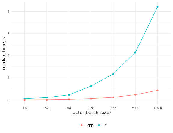
As we can see, the speed gain was significant, and catching up to C++ code through parallelizing R code is not feasible.
3. Iterators for exporting batches from the database
R has a well-deserved reputation as a language for processing data that fits into RAM, while Python is more characterized by iterative data processing that easily and effortlessly implements out-of-core computations (computations using external memory). A classic and relevant example for us in the context of the described task are deep neural networks trained using the gradient descent method with gradient approximation at each step using a small batch of observations, or mini-batch.
Deep learning frameworks written in Python have special classes that implement data iterators: for tables, images in directories, binary formats, etc. You can use existing options or write your own for specific tasks. In R, we can take advantage of all the features of the Python library keras with its various backends using the eponymous package, which in turn works on top of the package reticulate. The latter deserves a separate major article; it not only allows running Python code from R but also facilitates the transfer of objects between R and Python sessions, automatically performing all necessary type conversions.
We have eliminated the need to store all data in RAM by using MonetDBLite, all 'neural network' work will be done by the original Python code; we just need to write a data iterator, as there is no ready-made solution for this situation in either R or Python. There are essentially two requirements for it: it must return batches in an endless loop and maintain its state between iterations (the latter can be implemented in R simply using closures). Previously, it was necessary to explicitly convert R arrays to numpy arrays inside the iterator, but the current version of the package keras does this itself.
The iterator for training and validation data turned out as follows:
Iterator for training and validation data
train_generator <- function(db_connection = con,
                            samples_index,
                            num_classes = 340,
                            batch_size = 32,
                            scale = 1,
                            color = FALSE,
                            imagenet_preproc = FALSE) {
  # Проверка аргументов
  checkmate::assert_class(con, "DBIConnection")
  checkmate::assert_integerish(samples_index)
  checkmate::assert_count(num_classes)
  checkmate::assert_count(batch_size)
  checkmate::assert_number(scale, lower = 0.001, upper = 5)
  checkmate::assert_flag(color)
  checkmate::assert_flag(imagenet_preproc)

  # Перемешиваем, чтобы брать и удалять использованные индексы батчей по порядку
  dt <- data.table::data.table(id = sample(samples_index))
  # Проставляем номера батчей
  dt[, batch := (.I - 1L) %/% batch_size + 1L]
  # Оставляем только полные батчи и индексируем
  dt <- dt[, if (.N == batch_size) .SD, keyby = batch]
  # Устанавливаем счётчик
  i <- 1
  # Количество батчей
  max_i <- dt[, max(batch)]

  # Подготовка выражения для выгрузки
  sql <- sprintf(
    "PREPARE SELECT drawing, label_int FROM doodles WHERE id IN (%s)",
    paste(rep("?", batch_size), collapse = ",")
  )
  res <- DBI::dbSendQuery(con, sql)

  # Аналог keras::to_categorical
  to_categorical <- function(x, num) {
    n <- length(x)
    m <- numeric(n * num)
    m[x * n + seq_len(n)] <- 1
    dim(m) <- c(n, num)
    return(m)
  }

  # Замыкание
  function() {
    # Начинаем новую эпоху
    if (i > max_i) {
      dt[, id := sample(id)]
      data.table::setkey(dt, batch)
      # Сбрасываем счётчик
      i <<- 1
      max_i <<- dt[, max(batch)]
    }

    # ID для выгрузки данных
    batch_ind <- dt[batch == i, id]
    # Выгрузка данных
    batch <- DBI::dbFetch(DBI::dbBind(res, as.list(batch_ind)), n = -1)

    # Увеличиваем счётчик
    i <<- i + 1

    # Парсинг JSON и подготовка массива
    batch_x <- cpp_process_json_vector(batch$drawing, scale = scale, color = color)
    if (imagenet_preproc) {
      # Шкалирование c интервала [0, 1] на интервал [-1, 1]
      batch_x <- (batch_x - 0.5) * 2
    }

    batch_y <- to_categorical(batch$label_int, num_classes)
    result <- list(batch_x, batch_y)
    return(result)
  }
}
The function takes as input a variable with a connection to the database, the indices of the rows used, the number of classes, the batch size, the scale (scale = 1 corresponding to rendering images of 256x256 pixels, scale = 0.5 — 128x128 pixels), the color indicator (color = FALSE specifies rendering in shades of gray, when used color = TRUE each stroke is drawn with a new color) and a preprocessing indicator for networks pretrained on ImageNet. The latter is necessary to scale pixel values from the range [0, 1] to the range [-1, 1], which was used during the training of the provided models. keras models.
The external function includes argument type checks, a table data.table with randomly shuffled row numbers from samples_index and batch numbers, a counter and a maximum number of batches, as well as an SQL expression for extracting data from the database. Additionally, we defined a quick analog of the function keras::to_categorical(). We used almost all the data for training, leaving half a percent for validation, so the epoch size was limited by the parameter steps_per_epoch when calling keras::fit_generator(), and the condition if (i > max_i) triggered only for the validation iterator.
In the internal function, row indices for the next batch are sampled, records are extracted from the database with an increment of the batch counter, JSONs are parsed (the function cpp_process_json_vector(), written in C++) and arrays corresponding to the images are created. Then one-hot vectors with class labels, arrays with pixel values, and labels are combined into a list, which is the return value. To speed up the process, index creation in tables was used data.table and referenced modification — without these 'tricks' of the package data.table it is quite difficult to imagine efficient work with any significant amounts of data in R.
The results of the speed measurements on a laptop with a Core i5 look as follows:
Benchmark of the iterator
library(Rcpp)
library(keras)
library(ggplot2)

source("utils/rcpp.R")
source("utils/keras_iterator.R")

con <- DBI::dbConnect(drv = MonetDBLite::MonetDBLite(), Sys.getenv("DBDIR"))

ind <- seq_len(DBI::dbGetQuery(con, "SELECT count(*) FROM doodles")[[1L]])
num_classes <- DBI::dbGetQuery(con, "SELECT max(label_int) + 1 FROM doodles")[[1L]]

# Indices for the training set
train_ind <- sample(ind, floor(length(ind) * 0.995))
# Indices for the validation set
val_ind <- ind[-train_ind]
rm(ind)
# Scaling factor
scale <- 0.5

# Performance measurement
res_bench <- bench::press(
  batch_size = 2^(4:10),
  {
    it1 <- train_generator(
      db_connection = con,
      samples_index = train_ind,
      num_classes = num_classes,
      batch_size = batch_size,
      scale = scale
    )
    bench::mark(
      it1(),
      min_iterations = 50L
    )
  }
)
# Benchmark parameters
cols <- c("batch_size", "min", "median", "max", "itr/sec", "total_time", "n_itr")
res_bench[, cols]

#   batch_size      min   median      max `itr/sec` total_time n_itr
#
# 1         16     25ms  64.36ms   92.2ms     15.9       3.09s    49
# 2         32   48.4ms 118.13ms 197.24ms     8.17       5.88s    48
# 3         64   69.3ms 117.93ms 181.14ms     8.57       5.83s    50
# 4        128  157.2ms 240.74ms 503.87ms     3.85      12.71s    49
# 5        256  359.3ms 613.52ms 988.73ms     1.54       30.5s    47
# 6        512  884.7ms    1.53s    2.07s     0.674      1.11m    45
# 7       1024     2.7s    3.83s    5.47s     0.261      2.81m    44

ggplot(res_bench, aes(x = factor(batch_size), y = median, group = 1)) +
    geom_point() +
    geom_line() +
    ylab("median time, s") +
    theme_minimal()

DBI::dbDisconnect(con, shutdown = TRUE) 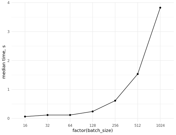
If there is enough RAM available, the database performance can be significantly enhanced by loading it into RAM (32 GB is sufficient for our task). In Linux, a partition is mounted by default, /dev/shm, taking up to half of the RAM. More can be allocated by editing /etc/fstab, so that it reads as tmpfs /dev/shm tmpfs defaults,size=25g 0 0. Be sure to restart and check the result by executing the command df -h.
The iterator for the test data is much simpler, as the entire test dataset fits into RAM:
Iterator for test data
test_generator <- function(dt,
                           batch_size = 32,
                           scale = 1,
                           color = FALSE,
                           imagenet_preproc = FALSE) {

  # Проверка аргументов
  checkmate::assert_data_table(dt)
  checkmate::assert_count(batch_size)
  checkmate::assert_number(scale, lower = 0.001, upper = 5)
  checkmate::assert_flag(color)
  checkmate::assert_flag(imagenet_preproc)

  # Проставляем номера батчей
  dt[, batch := (.I - 1L) %/% batch_size + 1L]
  data.table::setkey(dt, batch)
  i <- 1
  max_i <- dt[, max(batch)]

  # Замыкание
  function() {
    batch_x <- cpp_process_json_vector(dt[batch == i, drawing],
                                       scale = scale, color = color)
    if (imagenet_preproc) {
      # Шкалирование c интервала [0, 1] на интервал [-1, 1]
      batch_x <- (batch_x - 0.5) * 2
    }
    result <- list(batch_x)
    i <<- i + 1
    return(result)
  }
}
4. Choosing the model architecture
The first architecture used was , the details of which are discussed in the message. It is included in the standard distribution keras and is therefore available in the namesake package for R. However, when trying to use it with single-channel images, it was found that the input tensor must always have dimensions (batch, height, width, 3), meaning that the number of channels cannot be changed. In Python, there is no such limitation, so we rushed and wrote our own implementation of this architecture, following the original article (without the dropout that exists in the Keras version):
MobileNet V1 Architecture
library(keras)

top_3_categorical_accuracy <- custom_metric(
    name = "top_3_categorical_accuracy",
    metric_fn = function(y_true, y_pred) {
         metric_top_k_categorical_accuracy(y_true, y_pred, k = 3)
    }
)

layer_sep_conv_bn %
  layer_batch_normalization() %>%
  layer_activation_relu() %>%
  layer_conv_2d(
    filters = filters * alpha,
    kernel_size = c(1, 1),
    strides = c(1, 1)
  ) %>%
  layer_batch_normalization() %>%
  layer_activation_relu()
}

get_mobilenet_v1 <- function(input_shape = c(224, 224, 1),
                             num_classes = 340,
                             alpha = 1,
                             depth_multiplier = 1,
                             optimizer = optimizer_adam(lr = 0.002),
                             loss = "categorical_crossentropy",
                             metrics = c("categorical_crossentropy",
                                         top_3_categorical_accuracy)) {

  inputs <- layer_input(shape = input_shape)

  outputs %
    layer_conv_2d(filters = 32, kernel_size = c(3, 3), strides = c(2, 2), padding = "same") %>%
    layer_batch_normalization() %>%
    layer_activation_relu() %>%
    layer_sep_conv_bn(filters = 64, strides = c(1, 1)) %>%
    layer_sep_conv_bn(filters = 128, strides = c(2, 2)) %>%
    layer_sep_conv_bn(filters = 128, strides = c(1, 1)) %>%
    layer_sep_conv_bn(filters = 256, strides = c(2, 2)) %>%
    layer_sep_conv_bn(filters = 256, strides = c(1, 1)) %>%
    layer_sep_conv_bn(filters = 512, strides = c(2, 2)) %>%
    layer_sep_conv_bn(filters = 512, strides = c(1, 1)) %>%
    layer_sep_conv_bn(filters = 512, strides = c(1, 1)) %>%
    layer_sep_conv_bn(filters = 512, strides = c(1, 1)) %>%
    layer_sep_conv_bn(filters = 512, strides = c(1, 1)) %>%
    layer_sep_conv_bn(filters = 512, strides = c(1, 1)) %>%
    layer_sep_conv_bn(filters = 1024, strides = c(2, 2)) %>%
    layer_sep_conv_bn(filters = 1024, strides = c(1, 1)) %>%
    layer_global_average_pooling_2d() %>%
    layer_dense(units = num_classes) %>%
    layer_activation_softmax()

    model % compile(
      optimizer = optimizer,
      loss = loss,
      metrics = metrics
    )

    return(model)
}
The drawbacks of this approach are obvious. There are many models we want to test, but rewriting each architecture manually is undesirable. We also lost the ability to use weights from models pre-trained on ImageNet. As usual, studying the documentation helped. The function get_config() allows us to get a description of the model in an editable format (base_model_conf$layers — a regular R-style list), and the function from_config() performs a reverse transformation into a model object:
base_model_conf <- get_config(base_model)
base_model_conf$layers[[1]]$config$batch_input_shape[[4]] <- 1L
base_model <- from_config(base_model_conf)
Now it's easy to write a universal function for retrieving any of the models supplied with keras pre-trained weights on imagenet or without them:
Function to load ready-made architectures
get_model <- function(name = "mobilenet_v2",
                      input_shape = NULL,
                      weights = "imagenet",
                      pooling = "avg",
                      num_classes = NULL,
                      optimizer = keras::optimizer_adam(lr = 0.002),
                      loss = "categorical_crossentropy",
                      metrics = NULL,
                      color = TRUE,
                      compile = FALSE) {
  # Argument checks
  checkmate::assert_string(name)
  checkmate::assert_integerish(input_shape, lower = 1, upper = 256, len = 3)
  checkmate::assert_count(num_classes)
  checkmate::assert_flag(color)
  checkmate::assert_flag(compile)

  # Getting the object from the keras package
  model_fun <- get0(paste0("application_", name), envir = asNamespace("keras"))
  # Check for the object's existence in the package
  if (is.null(model_fun)) {
    stop("Model ", shQuote(name), " not found.", call. = FALSE)
  }

  base_model <- model_fun(
    input_shape = input_shape,
    include_top = FALSE,
    weights = weights,
    pooling = pooling
  )

  # If the image is not in color, change the input dimension
  if (!color) {
    base_model_conf <- keras::get_config(base_model)
    base_model_conf$layers[[1]]$config$batch_input_shape[[4]] <- 1L
    base_model <- keras::from_config(base_model_conf)
  }

  predictions <- keras::get_layer(base_model, "global_average_pooling2d_1")$output
  predictions <- keras::layer_dense(predictions, units = num_classes, activation = "softmax")
  model <- keras::keras_model(
    inputs = base_model$input,
    outputs = predictions
  )

  if (compile) {
    keras::compile(
      object = model,
      optimizer = optimizer,
      loss = loss,
      metrics = metrics
    )
  }

  return(model)
}
When using single-channel images, the pre-trained weights are not used. This could be fixed: using the function get_weights() to retrieve the model weights as a list of R arrays, change the dimension of the first element of that list (by taking one color channel or averaging all three), and then load the weights back into the model with the function set_weights(). We did not add this functionality since it had already become clear at this stage that it was more productive to work with color images.
Most of our experiments were conducted using mobilenet versions 1 and 2, as well as resnet34. In this competition, more modern architectures like SE-ResNeXt performed well. Unfortunately, we did not have any ready implementations available, and we have not written our own yet (but we will definitely do so).
5. Script Parameterization
For convenience, all the code for running the training was formatted as a single script, parameterized using as follows:
doc <- '
Usage:
  train_nn.R --help
  train_nn.R --list-models
  train_nn.R [options]

Options:
  -h --help                   Show this message.
  -l --list-models            List available models.
  -m --model=          Neural network model name [default: mobilenet_v2].
  -b --batch-size=      Batch size [default: 32].
  -s --scale-factor=   Scale factor [default: 0.5].
  -c --color                  Use color lines [default: FALSE].
  -d --db-dir=          Path to database directory [default: Sys.getenv("db_dir")].
  -r --validate-ratio= Validate sample ratio [default: 0.995].
  -n --n-gpu=         Number of GPUs [default: 1].
'
args <- docopt::docopt(doc)
The package docopt represents an implementation for R. With it, scripts are run using simple commands like Rscript bin/train_nn.R -m resnet50 -c -d /home/andrey/doodle_db or ./bin/train_nn.R -m resnet50 -c -d /home/andrey/doodle_db, if the file train_nn.R is executable (this command will start training the model resnet50 on three-channel images of size 128x128 pixels, the database should be in the folder /home/andrey/doodle_db). The list can include learning rate, optimizer type, and any other customizable parameters. During the preparation for publication, it became clear that the architecture mobilenet_v2 from the current version keras is not usable in R due to changes not accounted for in the R package — we are waiting for a fix.
This approach has significantly accelerated experiments with different models compared to the more traditional method of running scripts in RStudio (as a possible alternative, we note the package ). But the main advantage is the ability to easily manage script execution in Docker or simply on a server without installing RStudio for this purpose.
6. Dockerizing Scripts
We used Docker to ensure environment portability for model training among team members and for rapid deployment in the cloud. You can start getting acquainted with this relatively unfamiliar tool for R programmers with a series of publications or a .
Docker allows you to create your own images "from scratch" as well as use other images as a base for creating your own. After analyzing the available options, we concluded that installing NVIDIA drivers, CUDA+cuDNN, and Python libraries is a rather substantial part of the image, and we decided to base it on the official image tensorflow/tensorflow:1.12.0-gpu, adding the necessary R packages.
The final Dockerfile turned out as follows:
Dockerfile
FROM tensorflow/tensorflow:1.12.0-gpu

MAINTAINER Artem Klevtsov

SHELL ["/bin/bash", "-c"]

ARG LOCALE="en_US.UTF-8"
ARG APT_PKG="libopencv-dev r-base r-base-dev littler"
ARG R_BIN_PKG="futile.logger checkmate data.table rcpp rapidjsonr dbi keras jsonlite curl digest remotes"
ARG R_SRC_PKG="xtensor RcppThread docopt MonetDBLite"
ARG PY_PIP_PKG="keras"
ARG DIRS="/db /app /app/data /app/models /app/logs"

RUN source /etc/os-release &&
    echo "deb https://cloud.r-project.org/bin/linux/ubuntu ${UBUNTU_CODENAME}-cran35/" > /etc/apt/sources.list.d/cran35.list &&
    apt-key adv --keyserver keyserver.ubuntu.com --recv-keys E084DAB9 &&
    add-apt-repository -y ppa:marutter/c2d4u3.5 &&
    add-apt-repository -y ppa:timsc/opencv-3.4 &&
    apt-get update &&
    apt-get install -y locales &&
    locale-gen ${LOCALE} &&
    apt-get install -y --no-install-recommends ${APT_PKG} &&
    ln -s /usr/lib/R/site-library/littler/examples/install.r /usr/local/bin/install.r &&
    ln -s /usr/lib/R/site-library/littler/examples/install2.r /usr/local/bin/install2.r &&
    ln -s /usr/lib/R/site-library/littler/examples/installGithub.r /usr/local/bin/installGithub.r &&
    echo 'options(Ncpus = parallel::detectCores())' >> /etc/R/Rprofile.site &&
    echo 'options(repos = c(CRAN = "https://cloud.r-project.org"))' >> /etc/R/Rprofile.site &&
    apt-get install -y $(printf "r-cran-%s " ${R_BIN_PKG}) &&
    install.r ${R_SRC_PKG} &&
    pip install ${PY_PIP_PKG} &&
    mkdir -p ${DIRS} &&
    chmod 777 ${DIRS} &&
    rm -rf /tmp/downloaded_packages/ /tmp/*.rds &&
    rm -rf /var/lib/apt/lists/*

COPY utils /app/utils
COPY src /app/src
COPY tests /app/tests
COPY bin/*.R /app/

ENV DBDIR="/db"
ENV CUDA_HOME="/usr/local/cuda"
ENV PATH="/app:${PATH}"

WORKDIR /app

VOLUME /db
VOLUME /app

CMD bash
For convenience, the used packages were extracted into variables; the main part of the scripts is copied into the containers during the build. We also changed the command shell to /bin/bash for ease of using the contents /etc/os-release. This allowed us to avoid specifying the OS version in the code.
Additionally, a small bash script was written to allow running the container with various commands. For example, these could be scripts for training neural networks, previously placed inside the container, or a command shell for debugging and monitoring the operation of the container:
Script to run the container
#!/bin/sh

DBDIR=${PWD}/db
LOGSDIR=${PWD}/logs
MODELDIR=${PWD}/models
DATADIR=${PWD}/data
ARGS="--runtime=nvidia --rm -v ${DBDIR}:/db -v ${LOGSDIR}:/app/logs -v ${MODELDIR}:/app/models -v ${DATADIR}:/app/data"

if [ -z "$1" ]; then
    CMD="Rscript /app/train_nn.R"
elif [ "$1" = "bash" ]; then
    ARGS="${ARGS} -ti"
else
    CMD="Rscript /app/train_nn.R $@"
fi

docker run ${ARGS} doodles-tf ${CMD}
If this bash script is run without parameters, the default value script will be invoked inside the container. train_nn.R If the first positional argument is 'bash', the container will start in interactive mode with a command shell. In all other cases, the positional argument values will be substituted: CMD="Rscript /app/train_nn.R $@".
It should be noted that the directories containing the source data and database, as well as the directory for saving trained models, are mounted inside the container from the host system, allowing access to the results of script execution without unnecessary manipulations.
7. Using multiple GPUs on Google Cloud
One of the features of the competition was the quite noisy data (see the header image, borrowed from @Leigh.plt from ODS Slack). Battling this is aided by large batch sizes, and after experimenting on a PC with 1 GPU, we decided to master model training on multiple GPUs in the cloud. We used Google Cloud () due to the wide selection of available configurations, reasonable prices, and a $300 bonus. Out of greed, an instance with 4xV100 with SSD and a lot of RAM was ordered, and that was a big mistake. Such a machine consumes money quickly; without a well-prepared pipeline, one can go broke on experiments. For educational purposes, it's better to choose K80. However, the large amount of RAM came in handy — the cloud SSD did not impress with speed, so we carried the database to dev/shm.
The most interesting part of the code is responsible for using multiple GPUs. First, the model is created on the CPU using a context manager, just like in Python:
with(tensorflow::tf$device("/cpu:0"), {
  model_cpu <- get_model(
    name = model_name,
    input_shape = input_shape,
    weights = weights,
    metrics =(top_3_categorical_accuracy,
    compile = FALSE
  )
})
Then the uncompiled (this is important) model is copied to the specified number of available GPUs, and only after that is it compiled:
model <- keras::multi_gpu_model(model_cpu, gpus = n_gpu)
keras::compile(
  object = model,
  optimizer = keras::optimizer_adam(lr = 0.0004),
  loss = "categorical_crossentropy",
  metrics = c(top_3_categorical_accuracy)
)
The classic technique of freezing all layers except the last one, training the last layer, unfreezing, and retraining the model completely for multiple GPUs could not be implemented.
Training was monitored without using tensorboard, limiting ourselves to logging and saving models with informative names after each epoch:
Callbacks
# Шаблон имени файла лога
log_file_tmpl <- file.path("logs", sprintf(
  "%s_%d_%dch_%s.csv",
  model_name,
  dim_size,
  channels,
  format(Sys.time(), "%Y%m%d%H%M%OS")
))
# Шаблон имени файла модели
model_file_tmpl <- file.path("models", sprintf(
  "%s_%d_%dch_{epoch:02d}_{val_loss:.2f}.h5",
  model_name,
  dim_size,
  channels
))

callbacks_list <- list(
  keras::callback_csv_logger(
    filename = log_file_tmpl
  ),
  keras::callback_early_stopping(
    monitor = "val_loss",
    min_delta = 1e-4,
    patience = 8,
    verbose = 1,
    mode = "min"
  ),
  keras::callback_reduce_lr_on_plateau(
    monitor = "val_loss",
    factor = 0.5, # уменьшаем lr в 2 раза
    patience = 4,
    verbose = 1,
    min_delta = 1e-4,
    mode = "min"
  ),
  keras::callback_model_checkpoint(
    filepath = model_file_tmpl,
    monitor = "val_loss",
    save_best_only = FALSE,
    save_weights_only = FALSE,
    mode = "min"
  )
)
8. Instead of a conclusion
A number of problems we encountered have not yet been resolved:
- downward API support (simultaneously with this in keras there is no ready-made function for automatically finding the optimal learning rate (the equivalent of
lr_finderin the library fast.ai); with some effort, it is possible to port third-party implementations to R, for example, ; - as a consequence of the previous point, it was not possible to find the correct learning rate when using multiple GPUs;
- modern neural network architectures are lacking, especially those pre-trained on imagenet;
- there is no one cycle policy and discriminative learning rates (cosine annealing was introduced at our request, , thank you ).
What useful insights have we gained from this competition:
- On relatively low-power hardware, it is possible to work with substantial (greatly exceeding the size of RAM) datasets without difficulties. The package data.table saves memory by performing in-place modifications to tables, which avoids their copying, and when used correctly, it almost always demonstrates the highest speed among all known tools for scripting languages. Storing data in a database allows often not to worry about fitting the entire dataset into RAM.
- Slow functions in R can be replaced by fast ones in C++ using the package Rcpp. Additionally, using RcppThread or RcppParallel, we obtain cross-platform multithreaded implementations, so there is no need to parallelize the code at the R level.
- The package Rcpp can be used without serious knowledge of C++, the necessary minimum is described . Header files for several cool C libraries like xtensor are available on CRAN, creating an infrastructure for projects integrating high-performance C++ code into R. An additional convenience is the syntax highlighting and static code analyzer for C++ in RStudio.
- docopt allows running self-contained scripts with parameters. This is convenient for use on a remote server, including under Docker. Conducting long experiments with neural network training in RStudio is inconvenient, and installing the IDE on the server is not always justified.
- Docker provides code portability and reproducibility of results among developers with different OS versions and libraries, as well as ease of deployment on servers. You can launch the entire training pipeline with just one command.
- Google Cloud is a budget-friendly way to experiment on expensive hardware, but it's essential to choose configurations thoughtfully.
- Measuring the execution speed of individual code segments is very useful, especially when combining R and C++, and with the package bench it's also very easy.
Overall, this experience has been very valuable, and we continue working on addressing some of the mentioned issues.
Source: habr.com
