

Questa nota sarà interessante per coloro che utilizzano la libreria di elaborazione di dati tabulari per R — data.table, e potrebbe essere felice di vedere la flessibilità della sua applicazione attraverso diversi esempi.
Ispirandosi a un buon esempio , e sperando che abbiate già letto il suo articolo, propongo di approfondire l'ottimizzazione del codice e le prestazioni basate su data.table.
Introduzione: da dove proviene data.table?
È meglio iniziare ad avvicinarsi alla libreria da una certa distanza, ovvero dalle strutture dati da cui può essere ottenuto un oggetto data.table (d'ora in poi, DT).
Array
Codice
## arrays ---------

arrmatr <- array(1:20, c(4,5))

class(arrmatr)

typeof(arrmatr)

is.array(arrmatr)

is.matrix(arrmatr)
Una di queste strutture è l'array (?base::array). Come in altri linguaggi, gli array qui sono multidimensionali. Tuttavia, è interessante notare che, ad esempio, un array bidimensionale inizia a ereditare proprietà dalla classe matrice (?base::matrix), e un array monodimensionale, che è importante, non eredita da un vettore (?base::vector).
In tal modo va inteso che il tipo di dati contenuti in un oggetto deve essere verificato con la funzione base::typeof, che restituisce una descrizione interna del tipo secondo R Internals — un protocollo generale del linguaggio legato all'originario C.
Un'altra funzione, per determinare la classe di un oggetto, base::class, restituisce nel caso di vettori un tipo vettoriale (che si differenzia dal nome interno, ma consente anche di comprendere il tipo di dati).
Elenco
Da un array bidimensionale, ovvero una matrice, si può passare a una lista (?base::list).
Codice
## lists ------------------

mylist <- as.list(arrmatr)

is.vector(mylist)

is.list(mylist)
In tal modo accadono diverse cose simultaneamente:
- La seconda dimensione della matrice si riduce, cioè, otteniamo simultaneamente sia una lista che un vettore.
- La lista, così, eredita da queste classi. È importante tenere a mente che a un elemento della lista corrisponderà un valore (scalare) dalla cella della matrice-array.
Grazie al fatto che una lista è anche un vettore, si possono applicare ad essa alcune funzioni per vettori.
Dataframe
Da una lista, matrice o vettore si può passare a un dataframe (?base::data.frame).
Codice
## data.frames ------------

df <- as.data.frame(arrmatr)
df2 <- as.data.frame(mylist)

is.list(df)

df$V6 <- df$V1 + df$V2
Cosa c'è di interessante in esso: il dataframe eredita dalla lista! Le colonne del dataframe sono celle della lista. Questo sarà importante in seguito, quando utilizzeremo funzioni applicate alle liste.
data.table
Si può ottenere un DT (?data.table::data.table) da un dataframe, una lista, un vettore o una matrice. Ad esempio, in questo modo (in loco).
Codice
## data.tables -----------------------
library(data.table)

data.table::setDT(df)

is.list(df)

is.data.frame(df)

is.data.table(df)
È utile notare che, come il dataframe, il DT eredita le proprietà della lista.
DT e memoria
A differenza di tutti gli altri oggetti in R base, i data.table vengono passati per riferimento. Se è necessaria una copia in una nuova area di memoria, è necessaria una funzione data.table::copy oppure è necessario effettuare una selezione dall'oggetto originale.
Codice
df2 <- df

df[V1 == 1, V2 := 999]

data.table::fsetdiff(df, df2)

df2 <- data.table::copy(df)

df[V1 == 2, V2 := 999]

data.table::fsetdiff(df, df2)
Con questo, l'introduzione si conclude. I data.table rappresentano un'evoluzione delle strutture dati in R, che avviene principalmente attraverso l'ampliamento e l'accelerazione delle operazioni effettuate sugli oggetti della classe data.frame. In questo modo, si mantiene l'ereditarietà da altri primitivi.
Alcuni esempi di utilizzo delle proprietà dei data.table
Come una lista…
Iterare sulle righe di un data.frame o di un data.table non è la migliore idea, poiché il codice del ciclo in linguaggio R è di gran lunga più lento C, ma è possibile attraversare in ciclo le colonne, che di solito sono di gran lunga meno numerose. Percorrendo le colonne, ricordiamo che ogni colonna è un elemento di lista che contiene, di norma, un vettore. Le operazioni sui vettori sono ben vettorizzate nelle funzioni di base del linguaggio. Si possono anche utilizzare gli operatori di selezione caratteristici delle liste e dei vettori: `[[`, `$`.
Codice
## operations on data.tables ------------

#using list properties

df$'V1'[1]

df[['V1']]

df[[1]][1]

sapply(df, class)

sapply(df, function(x) sum(is.na(x)))
Vettorizzazione
Se è necessaria la percorrenza delle righe di un grande data.table, la soluzione migliore è scrivere una funzione con vettorizzazione. Ma se non fosse possibile, è importante ricordare che il ciclo all'interno è comunque più veloce del ciclo in R, poiché viene eseguito su C.
Proviamo con un esempio più grande con 100K righe. Estraiamo la prima lettera dalle parole che compongono la colonna vettore w.
Aggiornato
Codice
library(magrittr)
library(microbenchmark)

## Esempio più grande ----

rown <- 100000

dt %
	.[, d := 1 + b + c + rnorm(nrow(.))]

# vettorizzazione

microbenchmark({
	dt[
		, first_l := unlist(strsplit(w, split = ' ', fixed = T))[1]
		, by = 1:nrow(dt)
	   ]
})

# secondo

first_l_f %
		do.call(rbind, .) %>%
		`[`(,1)
}

dt[, first_l := NULL]

microbenchmark({
	dt[
		, first_l := .(first_l_f(w))
		]
})

# terzo

first_l_f2 %
		unlist %>%
		matrix(nrow = 3) %>%
		`[`(1,)
}

dt[, first_l := NULL]

microbenchmark({
	dt[
		, first_l := .(first_l_f2(w))
		]
})
Primo passaggio con iterazione sulle righe:
Unità: millisecondi
expr min
{ dt[, `:=`(first_l, unlist(strsplit(w, split = " ", fixed = T))[1]), by = 1:nrow(dt)] } 439.6217
lq media mediana uq max neval
451.9998 460.1593 456.2505 460.9147 621.4042 100
Secondo giro, dove la vettorizzazione avviene convertendo un elenco in una matrice e prelevando gli elementi da un taglio con indice 1 (quest'ultimo è propriamente la vettorizzazione). Mi correggo: la vettorizzazione a livello di funzione strsplit, che è in grado di accettare un vettore in ingresso. Si scopre che la procedura di conversione di un elenco in una matrice è molto più pesante della vettorizzazione stessa, ma in questo caso è comunque molto più veloce della variante non vettorizzata.
Unità: millisecondi
expr min lq mean median uq max neval
{ dt[, `:=`(first_l, .(first_l_f(w)))] } 93.07916 112.1381 161.9267 149.6863 185.9893 442.5199 100
Accelerazione per mediana in 3 volte.
Terzo giro, dove è stata modificata la procedura di conversione in matrice.
Unità: millisecondi
expr min lq mean median uq max neval
{ dt[, `:=`(first_l, .(first_l_f2(w)))] } 32.60481 34.13679 40.4544 35.57115 42.11975 222.972 100
Accelerazione per mediana in 13 volte.
Su questa questione bisogna sperimentare, più ne facciamo — meglio sarà.
Un altro esempio di vettorizzazione, dove è presente anche testo, ma è più vicino a condizioni reali: lunghezze diverse delle parole, numero variabile di parole. È necessario estrarre le prime 3 parole. Ecco come:
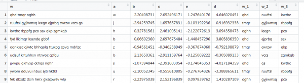
Qui la funzione precedente non funziona più, poiché i vettori sono di lunghezze diverse, e noi avevamo definito la dimensione della matrice. Riprogetteremo questa parte, cercando un po' su internet.
Codice
# fourth

rown <- 100000

words <-
	sapply(
		seq_len(rown)
		, function(x){
			nwords <- rbinom(1, 10, 0.5)
			paste(
				sapply(
					seq_len(nwords)
					, function(x){
						paste(sample(letters, rbinom(1, 10, 0.5), replace = T), collapse = '')
					}
				)
				, collapse = ' '
			)
		}
	)

dt <-
	data.table(
		w = words
		, a = sample(letters, rown, replace = T)
		, b = runif(rown, -3, 3)
		, c = runif(rown, -3, 3)
		, e = rnorm(rown)
	) %>%
	.[, d := 1 + b + c + rnorm(nrow(.))]

first_l_f3 <- function(sd, n)
{
	l <- strsplit(sd, split = ' ', fixed = T)

	maxl <- max(lengths(l))

	sapply(l, "length<-", maxl) %>%
		`[`(n,) %>%
		as.character
}

microbenchmark({
	dt[
		, (paste0('w_', 1:3)) := lapply(1:3, function(x) first_l_f3(w, x))
		]
})

dt[
	, (paste0('w_', 1:3)) := lapply(1:3, function(x) first_l_f3(w, x))
	]
Unità: millisecondi
expr min lq mean median
{ dt[, `:=`((paste0(«w_», 1:3)), strsplit(w, split = " ", fixed = T))] } 851.7623 916.071 1054.5 1035.199
uq max neval
1178.738 1356.816 100
Lo script ha funzionato con una velocità media di 1 secondo. Non male.
Collegati da una catena…
Con gli oggetti DT è possibile lavorare usando chaining. Questo appare come il collegamento della sintassi delle parentesi a destra, essenzialmente un dolcificante.
Codice
# chaining

res1 <- dt[a == 'a'][sample(.N, 100)]

res2 <- dt[, .N, a][, N]

res3 <- dt[, coefficients(lm(e ~ d))[1], a][, .(letter = a, coef = V1)]
Fluisce attraverso i tubi…
Operazioni simili possono essere eseguite tramite piping, che appare simile, ma è funzionalmente più ricco, poiché è possibile utilizzare qualsiasi metodo, non solo DT. Estraiamo i coefficienti di regressione logistica per i nostri dati sintetici con una serie di filtri su DT.
Codice
# piping

samplpe_b <- dt[a %in% head(letters), sample(b, 1)]

res4 <-
	dt %>%
	.[a %in% head(letters)] %>%
	.[,
	  {
	  	dt0 <- .SD[1:100]

	  	quants <-
	  		dt0[, c] %>%
	  		quantile(seq(0.1, 1, 0.1), na.rm = T)

	  	.(q = quants)
	  }
	  , .(cond = b > samplpe_b)
	  ] %>%
	glm(
		cond ~ q -1
		, family = binomial(link = "logit")
		, data = .
	) %>%
	summary %>%
	.[[12]]
Statistica, apprendimento automatico e altro all'interno di DT
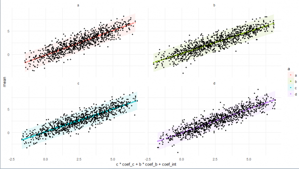
È possibile utilizzare funzioni lambda, ma a volte è meglio crearle separatamente, scrivere l'intero pipeline di analisi dei dati, e via — funzionano all'interno di DT. L'esempio è arricchito da tutte le funzionalità sopra elencate, più alcune cose utili dall'arsenale di DT (come l'accesso allo stesso DT all'interno di DT tramite collegamento, talvolta inserite non in sequenza, ma per completezza).
Codice
# function

rm(lm_preds)

lm_preds <- function(
	sd, by, n
)
{

	if(
		n < 100 |
		!by[['a']] %in% head(letters, 4)
	   )
	{

		res <-
			list(
				low = NA
				, mean = NA
				, high = NA
				, coefs = NA
			)

	} else {

		lmm <-
			lm(
				d ~ c + b
				, data = sd
			)

		preds <-
			stats::predict.lm(
				lmm
				, sd
				, interval = "prediction"
				)

		res <-
			list(
				low = preds[, 2]
				, mean = preds[, 1]
				, high = preds[, 3]
				, coefs = coefficients(lmm)
			)
	}

	res

}

res5 <-
	dt %>%
	.[e < 0] %>%
	.[.[, .I[b > 0]]] %>%
	.[, `:=` (
		low = as.numeric(lm_preds(.SD, .BY, .N)[[1]])
		, mean = as.numeric(lm_preds(.SD, .BY, .N)[[2]])
		, high = as.numeric(lm_preds(.SD, .BY, .N)[[3]])
		, coef_c = as.numeric(lm_preds(.SD, .BY, .N)[[4]][1])
		, coef_b = as.numeric(lm_preds(.SD, .BY, .N)[[4]][2])
		, coef_int = as.numeric(lm_preds(.SD, .BY, .N)[[4]][3])
	)
	, a
	] %>%
	.[!is.na(mean), -'e', with = F]


# plot

plo <-
	res5 %>%
	ggplot +
	facet_wrap(~ a) +
	geom_ribbon(
		aes(
			x = c * coef_c + b * coef_b + coef_int
			, ymin = low
			, ymax = high
			, fill = a
		)
		, size = 0.1
		, alpha = 0.1
	) +
	geom_point(
		aes(
			x = c * coef_c + b * coef_b + coef_int
			, y = mean
			, color = a
		)
		, size = 1
	) +
	geom_point(
		aes(
			x = c * coef_c + b * coef_b + coef_int
			, y = d
		)
		, size = 1
		, color = 'black'
	) +
	theme_minimal()

print(plo)
Conclusione
Spero di aver creato un quadro unitario ma, ovviamente, non completo, di un oggetto come data.table, partendo dalle sue proprietà legate all'ereditarietà delle classi R e giungendo alle sue peculiari caratteristiche e all'ambiente degli elementi tidyverse. Spero che questo ti aiuti a studiare e applicare meglio questa libreria per lavoro e divertimento.
Grazie!
Codice completo
Codice
## load libs ----------------

library(data.table)
library(ggplot2)
library(magrittr)
library(microbenchmark)


## arrays ---------

arrmatr <- array(1:20, c(4,5))

class(arrmatr)

typeof(arrmatr)

is.array(arrmatr)

is.matrix(arrmatr)


## lists ------------------

mylist <- as.list(arrmatr)

is.vector(mylist)

is.list(mylist)


## data.frames ------------

df <- as.data.frame(arrmatr)

is.list(df)

df$V6 <- df$V1 + df$V2


## data.tables -----------------------

data.table::setDT(df)

is.list(df)

is.data.frame(df)

is.data.table(df)

df2 <- df

df[V1 == 1, V2 := 999]

data.table::fsetdiff(df, df2)

df2 <- data.table::copy(df)

df[V1 == 2, V2 := 999]

data.table::fsetdiff(df, df2)


## operations on data.tables ------------

#using list properties

df$'V1'[1]

df[['V1']]

df[[1]][1]

sapply(df, class)

sapply(df, function(x) sum(is.na(x)))


## Bigger example ----

rown <- 100000

dt <-
	data.table(
		w = sapply(seq_len(rown), function(x) paste(sample(letters, 3, replace = T), collapse = ' '))
		, a = sample(letters, rown, replace = T)
		, b = runif(rown, -3, 3)
		, c = runif(rown, -3, 3)
		, e = rnorm(rown)
	) %>%
	.[, d := 1 + b + c + rnorm(nrow(.))]

# vectorization

# zero - for loop

microbenchmark({
	for(i in 1:nrow(dt))
		{
		dt[
			i
			, first_l := unlist(strsplit(w, split = ' ', fixed = T))[1]
		]
	}
})

# first

microbenchmark({
	dt[
		, first_l := unlist(strsplit(w, split = ' ', fixed = T))[1]
		, by = 1:nrow(dt)
	   ]
})

# second

first_l_f <- function(sd)
{
	strsplit(sd, split = ' ', fixed = T) %>%
		do.call(rbind, .) %>%
		`[`(,1)
}

dt[, first_l := NULL]

microbenchmark({
	dt[
		, first_l := .(first_l_f(w))
		]
})

# third

first_l_f2 <- function(sd)
{
	strsplit(sd, split = ' ', fixed = T) %>%
		unlist %>%
		matrix(nrow = 3) %>%
		`[`(1,)
}

dt[, first_l := NULL]

microbenchmark({
	dt[
		, first_l := .(first_l_f2(w))
		]
})

# fourth

rown <- 100000

words <-
	sapply(
		seq_len(rown)
		, function(x){
			nwords <- rbinom(1, 10, 0.5)
			paste(
				sapply(
					seq_len(nwords)
					, function(x){
						paste(sample(letters, rbinom(1, 10, 0.5), replace = T), collapse = '')
					}
				)
				, collapse = ' '
			)
		}
	)

dt <-
	data.table(
		w = words
		, a = sample(letters, rown, replace = T)
		, b = runif(rown, -3, 3)
		, c = runif(rown, -3, 3)
		, e = rnorm(rown)
	) %>%
	.[, d := 1 + b + c + rnorm(nrow(.))]

first_l_f3 <- function(sd, n)
{
	l <- strsplit(sd, split = ' ', fixed = T)

	maxl <- max(lengths(l))

	sapply(l, "length<-", maxl) %>%
		`[`(n,) %>%
		as.character
}

microbenchmark({
	dt[
		, (paste0('w_', 1:3)) := lapply(1:3, function(x) first_l_f3(w, x))
		]
})

dt[
	, (paste0('w_', 1:3)) := lapply(1:3, function(x) first_l_f3(w, x))
	]


# chaining

res1 <- dt[a == 'a'][sample(.N, 100)]

res2 <- dt[, .N, a][, N]

res3 <- dt[, coefficients(lm(e ~ d))[1], a][, .(letter = a, coef = V1)]

# piping

samplpe_b <- dt[a %in% head(letters), sample(b, 1)]

res4 <-
	dt %>%
	.[a %in% head(letters)] %>%
	.[,
	  {
	  	dt0 <- .SD[1:100]

	  	quants <-
	  		dt0[, c] %>%
	  		quantile(seq(0.1, 1, 0.1), na.rm = T)

	  	.(q = quants)
	  }
	  , .(cond = b > samplpe_b)
	  ] %>%
	glm(
		cond ~ q -1
		, family = binomial(link = "logit")
		, data = .
	) %>%
	summary %>%
	.[[12]]


# function

rm(lm_preds)

lm_preds <- function(
	sd, by, n
)
{

	if(
		n < 100 |
		!by[['a']] %in% head(letters, 4)
	   )
	{

		res <-
			list(
				low = NA
				, mean = NA
				, high = NA
				, coefs = NA
			)

	} else {

		lmm <-
			lm(
				d ~ c + b
				, data = sd
			)

		preds <-
			stats::predict.lm(
				lmm
				, sd
				, interval = "prediction"
				)

		res <-
			list(
				low = preds[, 2]
				, mean = preds[, 1]
				, high = preds[, 3]
				, coefs = coefficients(lmm)
			)
	}

	res

}

res5 <-
	dt %>%
	.[e < 0] %>%
	.[.[, .I[b > 0]]] %>%
	.[, `:=` (
		low = as.numeric(lm_preds(.SD, .BY, .N)[[1]])
		, mean = as.numeric(lm_preds(.SD, .BY, .N)[[2]])
		, high = as.numeric(lm_preds(.SD, .BY, .N)[[3]])
		, coef_c = as.numeric(lm_preds(.SD, .BY, .N)[[4]][1])
		, coef_b = as.numeric(lm_preds(.SD, .BY, .N)[[4]][2])
		, coef_int = as.numeric(lm_preds(.SD, .BY, .N)[[4]][3])
	)
	, a
	] %>%
	.[!is.na(mean), -'e', with = F]


# plot

plo <-
	res5 %>%
	ggplot +
	facet_wrap(~ a) +
	geom_ribbon(
		aes(
			x = c * coef_c + b * coef_b + coef_int
			, ymin = low
			, ymax = high
			, fill = a
		)
		, size = 0.1
		, alpha = 0.1
	) +
	geom_point(
		aes(
			x = c * coef_c + b * coef_b + coef_int
			, y = mean
			, color = a
		)
		, size = 1
	) +
	geom_point(
		aes(
			x = c * coef_c + b * coef_b + coef_int
			, y = d
		)
		, size = 1
		, color = 'black'
	) +
	theme_minimal()

print(plo)
Fonte: habr.com
